L01 — Introduction to Machine Learning

Back to MPL Index | Next: (y-02) CNNs

Introduction

Machine perception is the capability of a computer system to interpret data in a manner similar to the way humans use their senses to relate to the world around them.

Machine learning provides systems with the ability to automatically learn and improve from experience without being explicitly programmed.

I use the SlideLink tool I built to automatically align these notes with the original lecture slides.

This course is in-depth, hands-on, and advanced — it assumes prior exposure to machine learning, deep learning, reinforcement learning, or computer vision.

---

Mental Model First

• This lecture introduces the full training loop: represent the input, measure how wrong the model is with a loss, then use gradients to improve the weights.
• A hidden layer is best thought of as a feature builder. Early layers turn raw numbers into useful intermediate patterns; later layers combine those patterns into decisions.
• Backpropagation is not “the network thinking backwards.” It is just a systematic way of assigning credit and blame to each parameter.
• If one question guides your reading, let it be this: how do simple mathematical blocks become a trainable system that improves from data?

Refresher: Neural Networks

The Perceptron

The basic unit of a neural network:

$y=\sigma (w^{\top }x+b)$

where:

• $w$ = weight vector
• $x$ = input
• $b$ = bias
• $\sigma$ = activation function

Multi-Layer Perceptron (MLP)

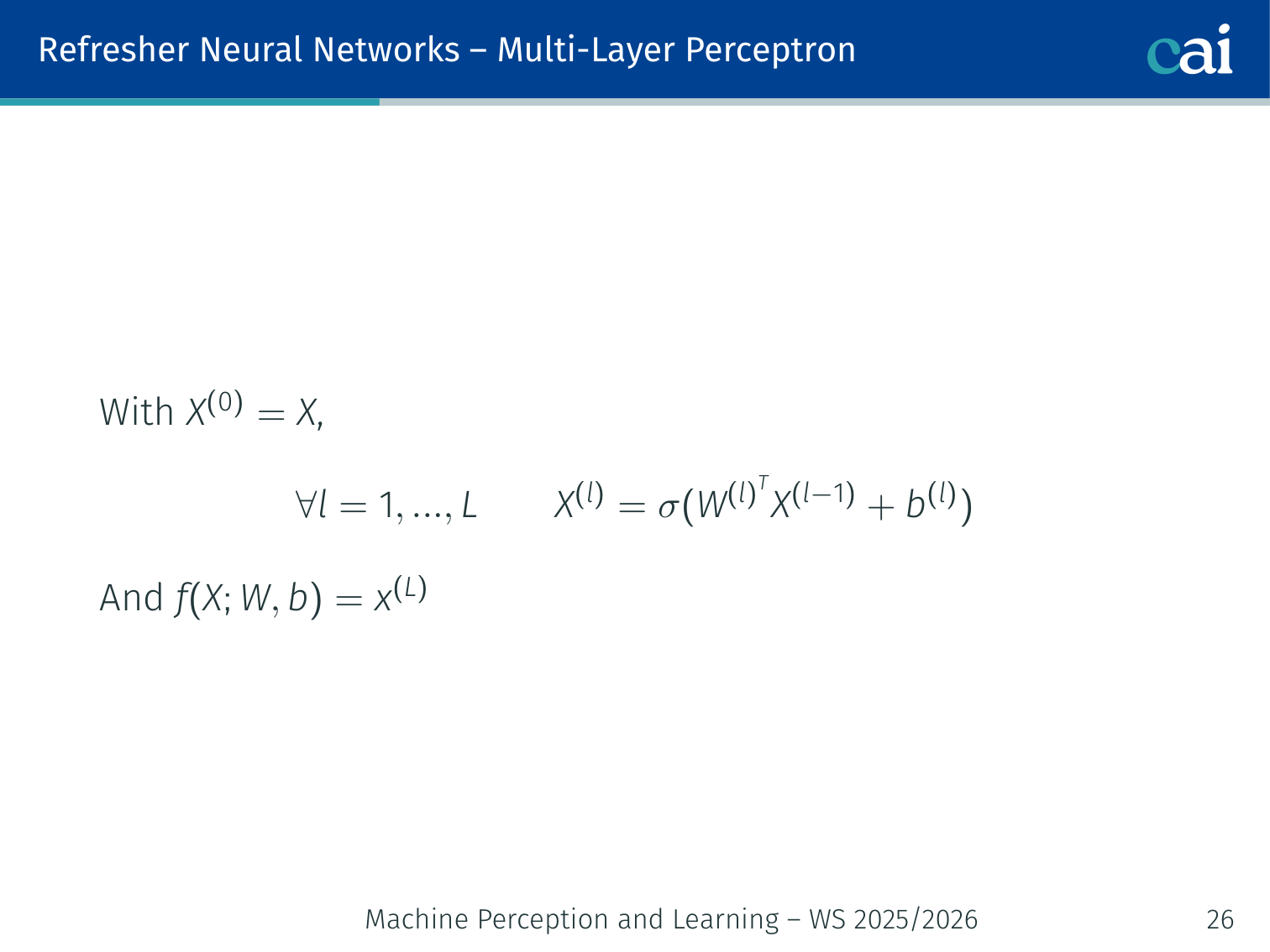
A basic MLP with layers stacked on top of each other.

With $X^{(0)}=X$, for each layer $l=1,\dots ,L$:

$X^{(l)}=\sigma \left(W^{(l)\top }{X}^{(l-1)}+b^{(l)}\right)$

The network output is $f(X;W,b)=X^{(L)}$.

💡 Intuition: What a Hidden Layer Is Really Doing

A hidden layer is easier to understand if you stop thinking about “neurons” and think about new coordinates.

• The raw input $x$ might be pixels, sensor values, or tabular features.
• The first hidden layer asks many small questions about that input: “is there an edge here?”, “is this value unusually large?”, “do these two features occur together?”
• The next layer works on those answers instead of the raw input directly.

So the network is gradually rewriting the problem into a space where the final decision becomes easier. Classification is often hard in pixel space, but much easier in a learned feature space.

Why Activation Functions?

Nonlinear activations are what let us learn complex patterns.

Moving from a linear classifier $f=Wx$ to a 2-layer network:

$f=W_2\max (0,W_{1}x),x\in {\mathbb{R}}^D,W_1\in {\mathbb{R}}^H\times D,W_2\in {\mathbb{R}}^C\times H$

Or a 3-layer network:

$f=W_3\max (0,W_2\max (0,W_{1}x))$

Without a non-linear activation: $f=W_2{W}_{1}x=W_{3}x$ — we collapse back to a linear classifier. Non-linearity is essential.

Brain Analogy — Be Careful

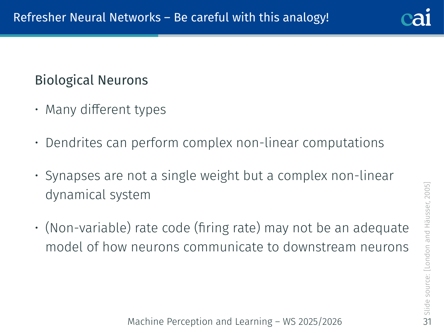
The brain analogy is a good start, but real neurons are way more complex.

Biological neurons ≠ artificial neurons:

• There are many different types of biological neurons
• Synapses are not a single weight but a complex non-linear dynamical system
• The firing-rate code may not adequately model inter-neuron communication
• Dendrites can perform complex non-linear computations

Universal Approximation Theorem

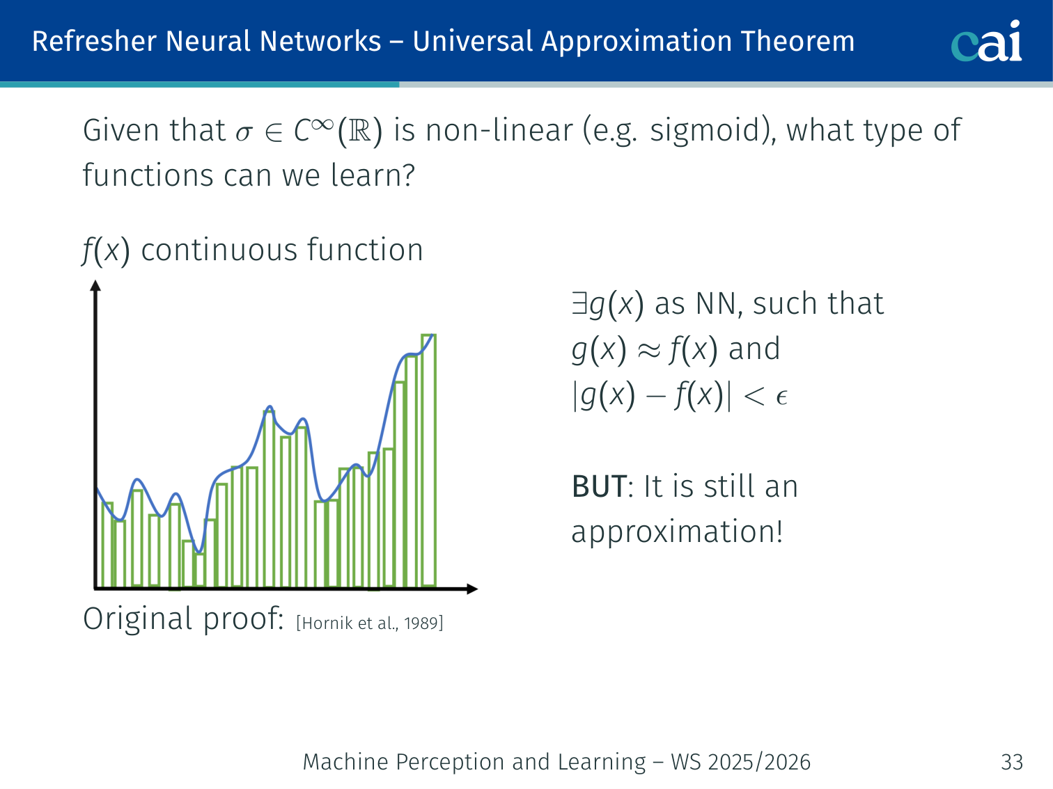
The math says even a shallow network can model any continuous function.

Given a non-linear (e.g. sigmoid) activation function $\sigma \in C^{\infty }(\mathbb{R})$, for any continuous function $f\in C(I^m)$ and any $\epsilon >0$, there exist $N$, constants ${\nu }_i,b_i\in \mathbb{R}$, and vectors $w_i\in {\mathbb{R}}^m$ such that:

$f(x)\approx g(x)={\sum }_{i=1}^N{\nu }_i\sigma (w_i^{\top }x+b_i),|g(x)-f(x)|<\epsilon \forall x\in I^m$

(Original proof: Hornik et al., 1989; formal statement: Cybenko, 1989)

Key intuition — building a “bump” function:

1. Increase weight $w$ until $\sigma (w^{\top }x+b)$ becomes a step function; step position $s=-b/w$
2. Two neurons (with step positions $s_1$, $s_2$) combine to form a “bump” of height $h$
3. Many such bump pairs can approximate any shape

Critical caveats:

• Networks with a single hidden layer need exponentially wide layers → in practice, deeper networks work better
• The theorem guarantees expressiveness, not learnability — it says nothing about whether gradient descent will find those weights

---

Optimisation

Optimizing is just about finding the weights that make the loss as small as possible.

The loss function $L(W)$ quantifies the quality of any set of weights $W$. The goal of optimisation is to find $W$ that minimises $L(W)$.

$L(W)=\frac{1}{n}{\sum }_{i=1}^n{L}_i(W)$

Gradient Descent

Gradient descent works by taking small steps downhill to find the minimum.

Strategy 1 — Random search: bad idea in practice.

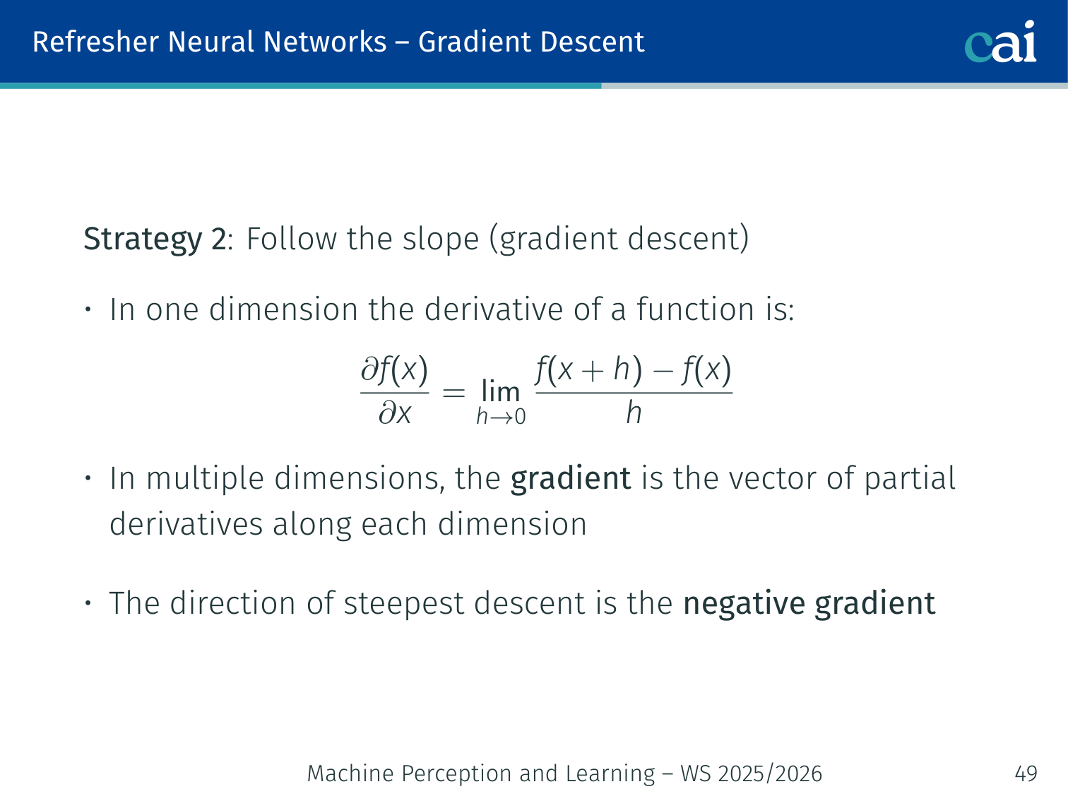
Strategy 2 — Follow the slope (gradient descent):

In one dimension, the derivative is: $\frac{\partial f(x)}{\partial x}={\lim }_{h\to 0}\frac{f(x+h)-f(x)}{h}$

In multiple dimensions, the gradient is the vector of partial derivatives along each dimension. The direction of steepest descent is the negative gradient.

Update rule (starting from $W_0$): $W_{t+1}=W_t-{\alpha }_t\nabla f(W_t)$

while True:
    weights_grad = evaluate_gradient(loss_fun, data, weights)
    weights += -step_size * weights_grad

Numerical vs. Analytic Gradient

Comparing numerical and analytic gradients for speed and accuracy.

Type	Description	Properties
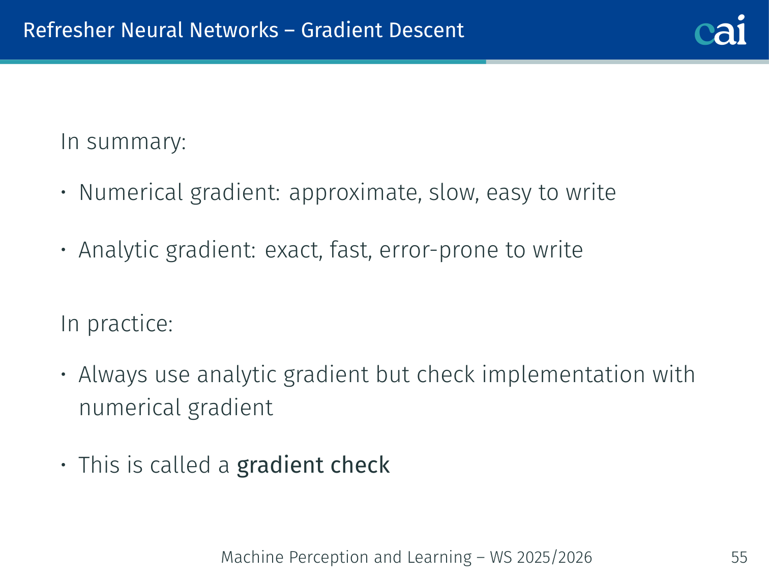
Numerical	$\frac{f(W+h)-f(W)}{h}$, computed per dimension	Approximate, slow, easy to write
Analytic	Exact derivative via calculus/backprop	Exact, fast, error-prone to implement

In practice: always use the analytic gradient, but verify your implementation with a gradient check using the numerical gradient.

Batch Training

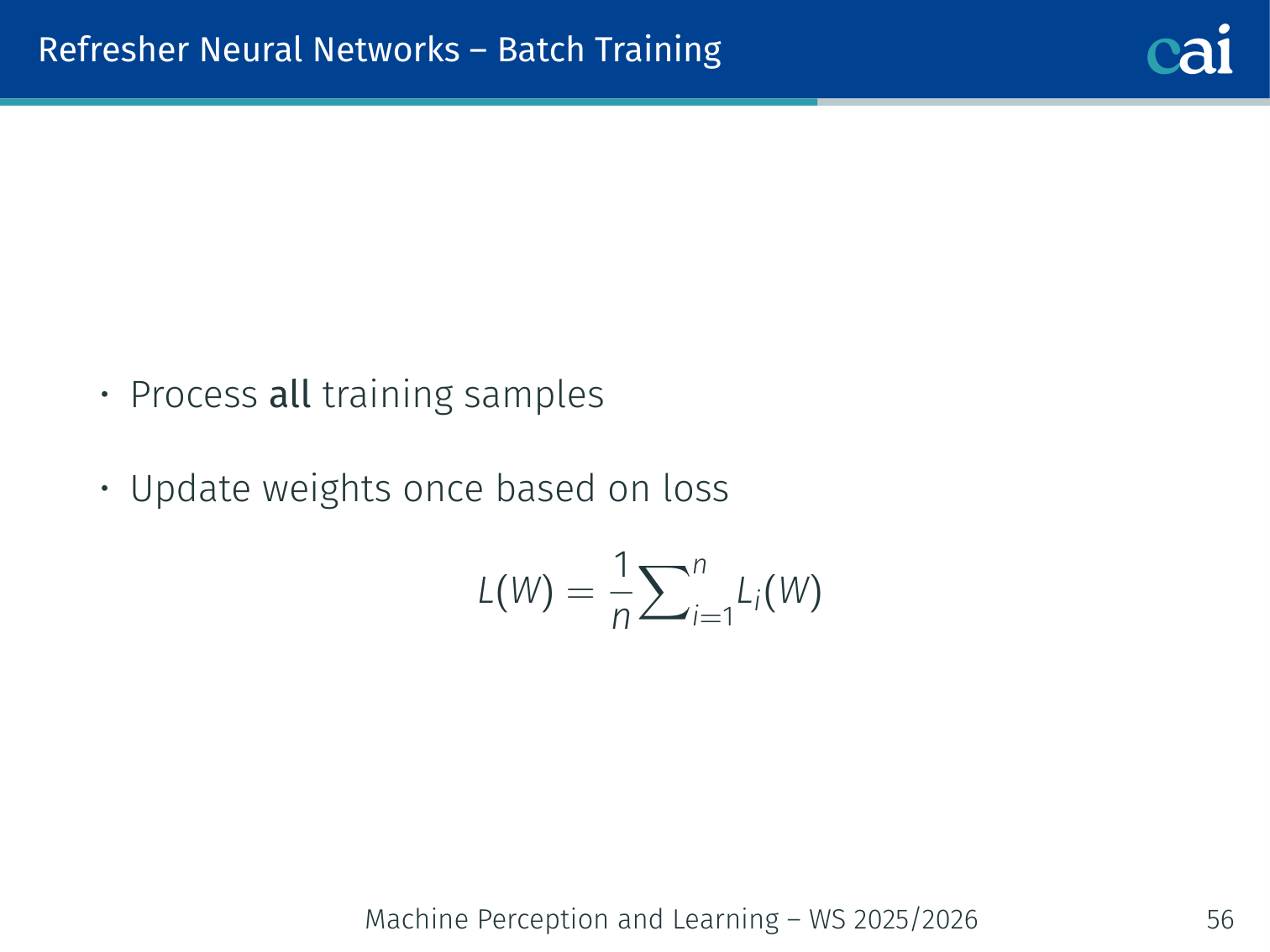
Batch training looks at every single sample before making one update.

Process all $n$ training samples, then update weights once based on $L(W)=\frac{1}{n}{\sum }_{i=1}^n{L}_i(W)$.

Upsides	Downsides
Fewer updates → higher computational efficiency	Stable gradient may cause premature convergence
Stable error gradient → more stable convergence	Requires entire training dataset in memory
Separates prediction and update → parallelisable	Very slow for large datasets

Stochastic Gradient Descent (SGD)

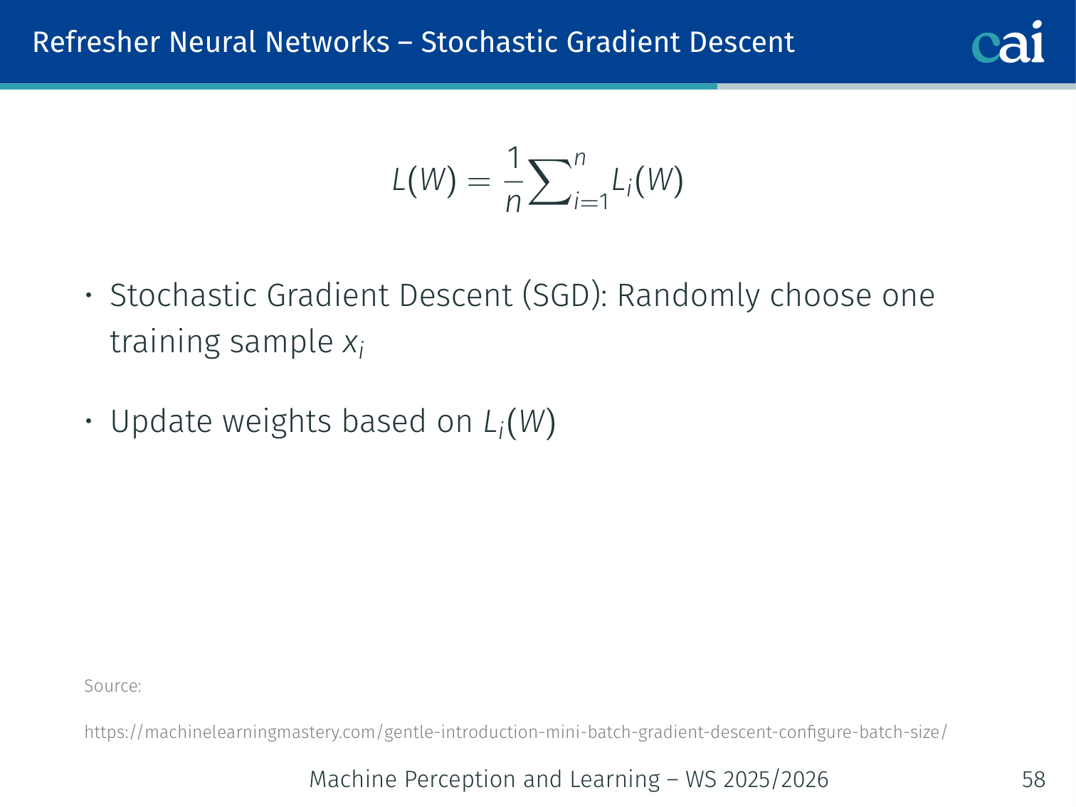
SGD updates the weights after every single example it sees.

Randomly choose one training sample $x_i$, update weights based on $L_i(W)$.

Upsides	Downsides
Frequent updates → insight into model performance	Computationally more expensive per epoch
Easy to understand and implement	Noisy gradient → parameters jump around (high variance)
Higher update frequency → faster learning on some problems	Hard for the algorithm to settle on a minimum
Noisy updates can escape local minima → robustness

Mini-Batch Training

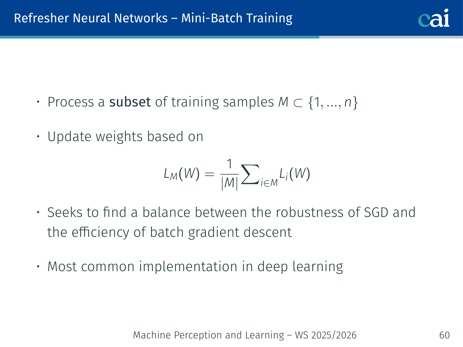
Mini-batches give us a nice balance between speed and stable updates.

Process a subset $M\subset \{1,\dots ,n\}$ of samples:

$L_M(W)=\frac{1}{|M|}{\sum }_{i\in M}{L}_i(W)$

Seeks a balance between the robustness of SGD and the efficiency of batch gradient descent. Most common implementation in deep learning.

Upsides	Downsides
Higher update frequency than batch → avoids local minima	Requires an extra hyperparameter (mini-batch size)
More computationally efficient than SGD	Error must be accumulated across mini-batches
Doesn’t require all data in memory

Backpropagation

Backprop uses the chain rule to figure out how much each weight contributed to the error.

How do we compute gradients for nodes in hidden layers? → Backpropagation applies the chain rule repeatedly from the output back to each parameter.

Computational Graphs

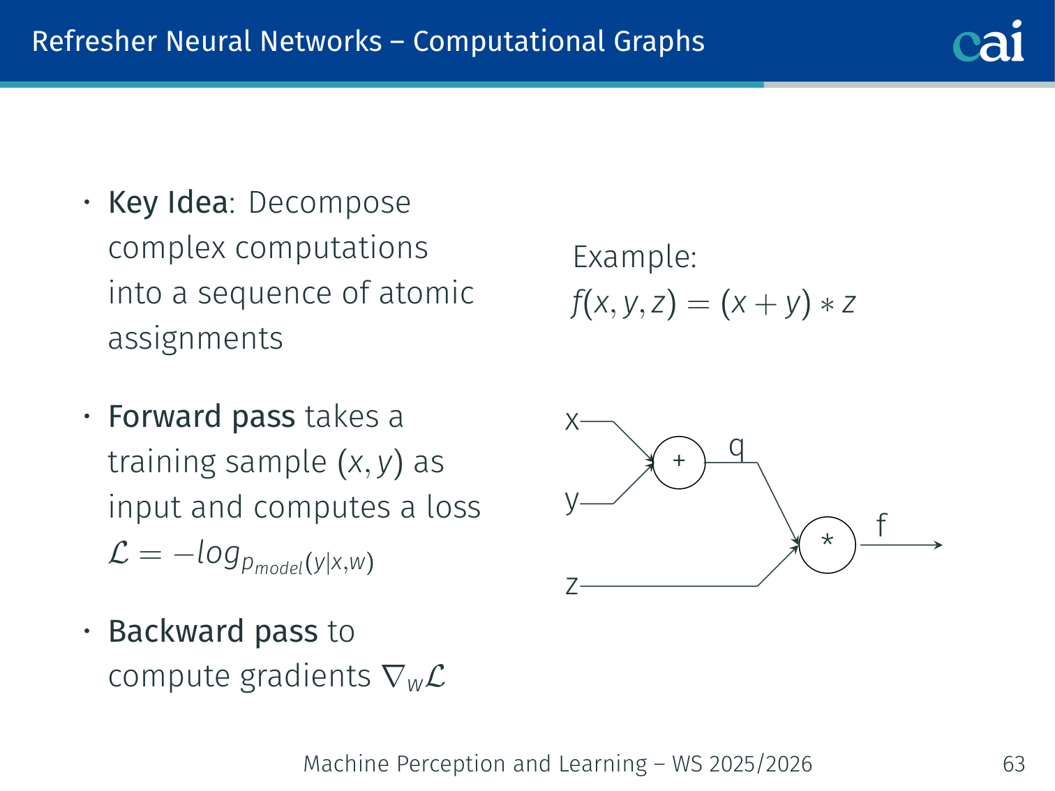
Computational graphs turn complex math into a sequence of simple, doable steps.

Key idea: decompose complex computations into a sequence of atomic assignments.

Example: $f(x,y,z)=(x+y)\cdot z$

x ──┐
    +──→ q ──┐
y ──┘         * ──→ f
z ────────────┘

• Forward pass: takes a training sample $(x,y)$ as input and computes loss $L=-\log p_{\text{model}}(y\mid x,w)$
• Backward pass: computes gradients ${\nabla }_{w}L$ via the chain rule

Worked example with $x=-2,y=5,z=-4$:

• $q=x+y=3$
• $f=q\cdot z=-12$
• $\frac{\partial f}{\partial z}=q=3$; $\frac{\partial f}{\partial q}=z=-4$
• $\frac{\partial f}{\partial x}=\frac{\partial f}{\partial q}\cdot 1=-4$; $\frac{\partial f}{\partial y}=-4$

💡 Intuition: Finding Your Way in the Dark

Imagine you are at the top of a mountain (the current loss) at night. You can’t see the bottom, but you can feel the slope of the ground under your feet.

• The Gradient: The direction of the steepest slope.
• Gradient Descent: Taking a small step in the opposite direction (downward).
• Learning Rate: How big your step is.
  • Too small? It takes forever to get home.
  • Too large? You might jump over the valley and end up on another mountain peak.

🧠 Deep Dive: Backpropagation Pattern Intuition

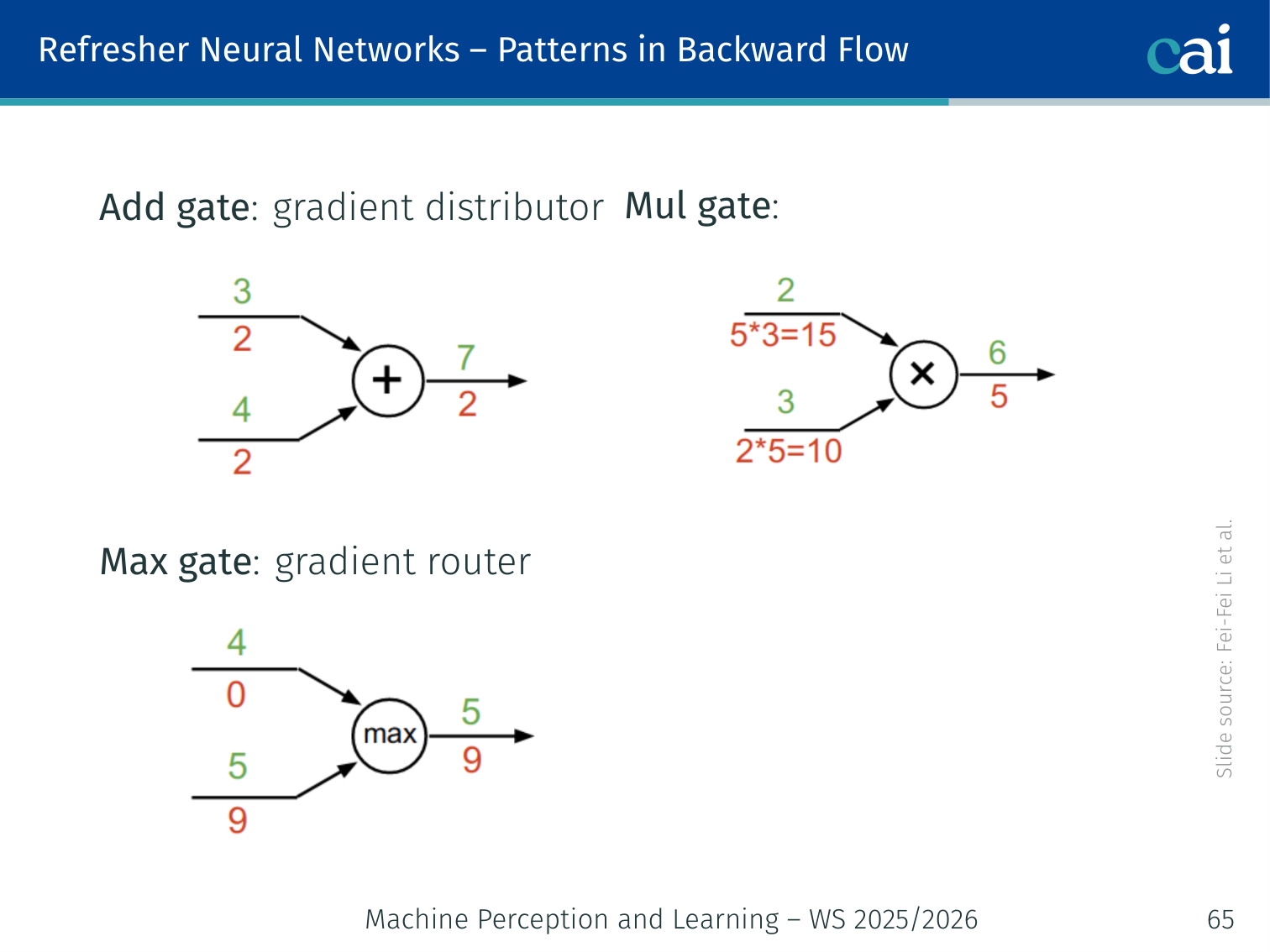
During the backward pass, each gate acts as a “gradient router”:

1. Add Gate (+): It is a Distributor. It sends the same gradient to both branches.
2. Mul Gate (*): It is a Scaler. It scales the gradient by the value of the other branch.
3. Max Gate: It is a Switch. It sends all the gradient to the branch that won, and zero to the others.

Why is this helpful?

• If your gradient is vanishing, you can look at your multiplication gates. If one branch is very small, it will kill the signal for the other branch.
• This is exactly why we normalize weights and use BatchNorm: to keep the values in a range where the “Scalers” (multiplication gates) don’t shrink the signal to zero.

---

Patterns in Backward Flow

Here’s how gradients flow through addition, multiplication, and max operations.

Gate	Role	Behaviour
Add gate	Gradient distributor	Passes the upstream gradient equally to both inputs
Max gate	Gradient router	Passes the upstream gradient to whichever input was larger; zero to the other
Mul gate	Gradient scaler	Passes upstream gradient × the other input’s value

---

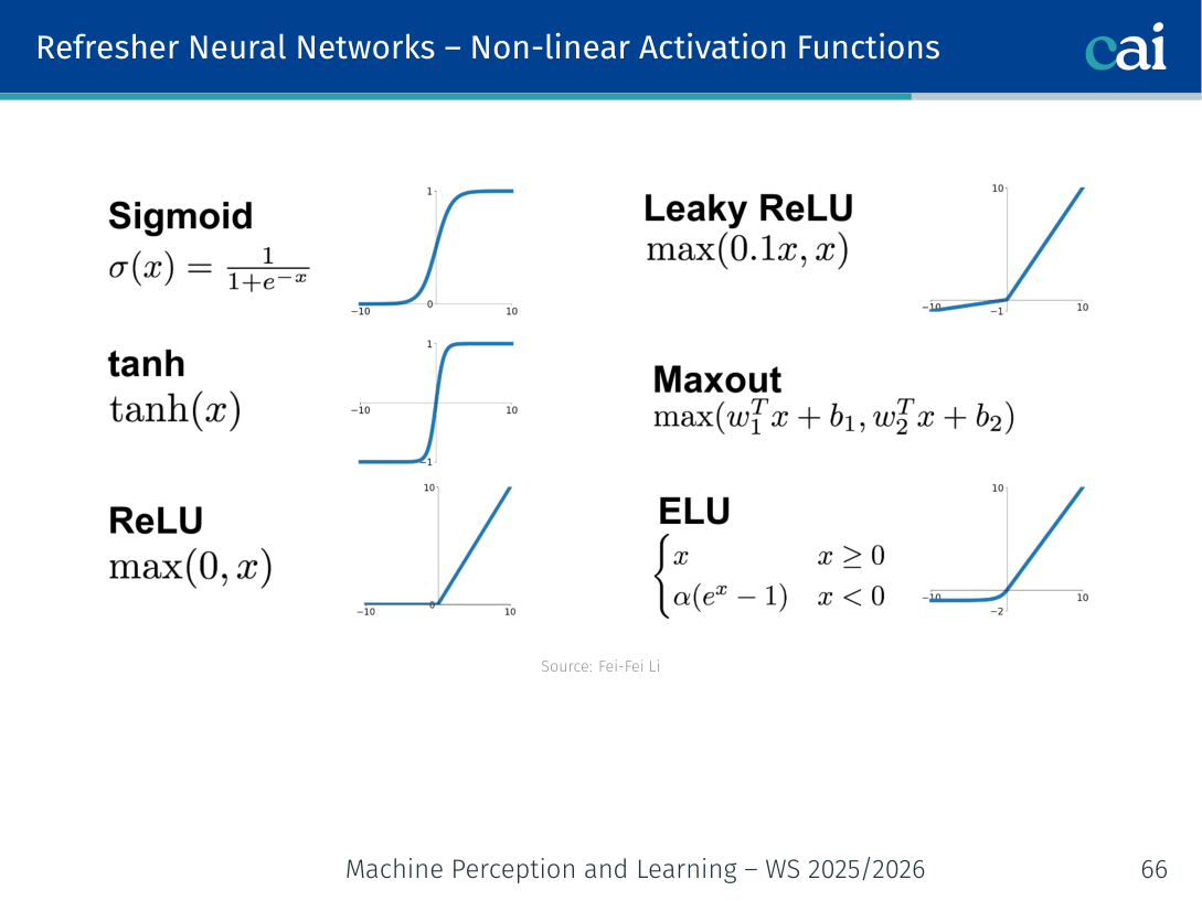
Activation Functions

Sigmoid

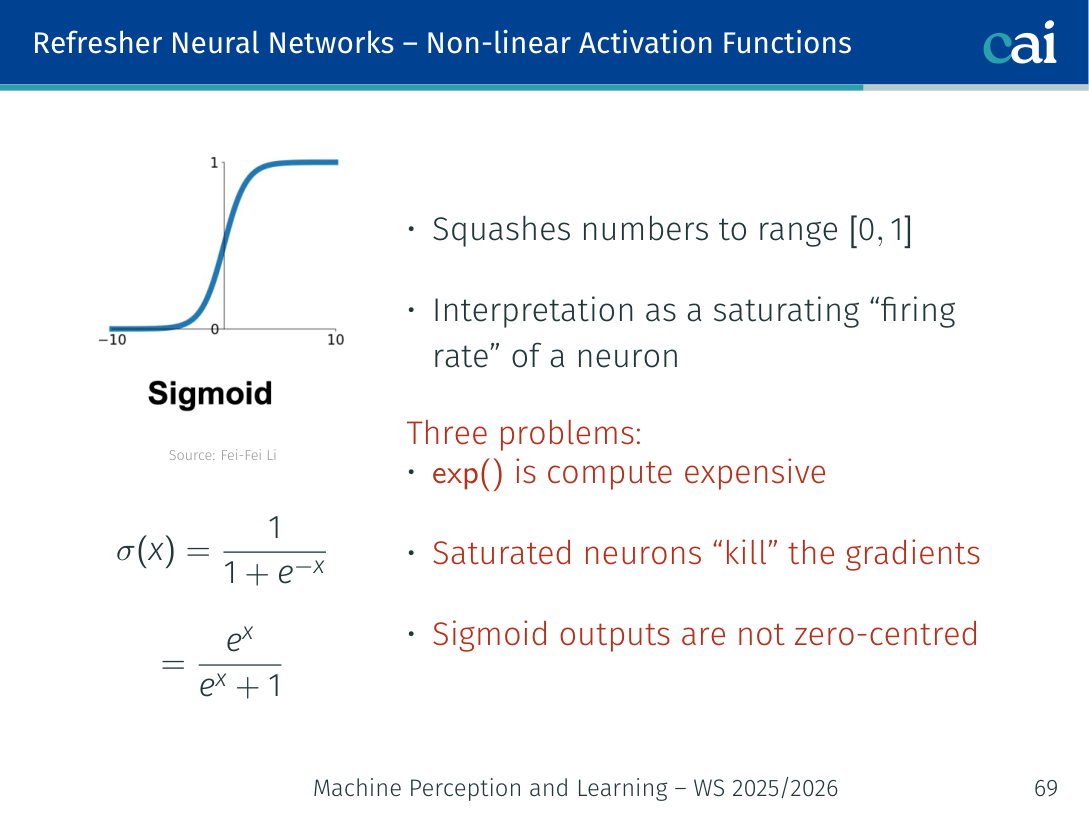
Sigmoid squashes everything between 0 and 1, but it can make gradients disappear.

$\sigma (x)=\frac{1}{1+e^{-x}}=\frac{e^x}{e^x+1}$

Squashes numbers to $[0,1]$. Can be interpreted as a saturating “firing rate” of a neuron.

Three problems:

1. Saturated neurons kill the gradients

   • $\frac{\partial \sigma }{\partial x}=\sigma (x)(1-\sigma (x))$
   • When $x=-10$: $\sigma (x)\approx 0\Rightarrow \frac{\partial \sigma }{\partial x}\approx 0$
   • When $x=10$: $\sigma (x)\approx 1\Rightarrow \frac{\partial \sigma }{\partial x}\approx 0$
   • Gradient vanishes → no learning signal propagates back

2. Sigmoid outputs are not zero-centred

   • Outputs always in $(0,1)$, so all upstream inputs to the next layer are positive
   • The gradient $\frac{\partial L}{\partial w_i}$ will all have the same sign as the upstream gradient → zig-zagging weight updates
   • Mini-batches or zero-mean data can partially mitigate this

3. exp() is computationally expensive

Tanh

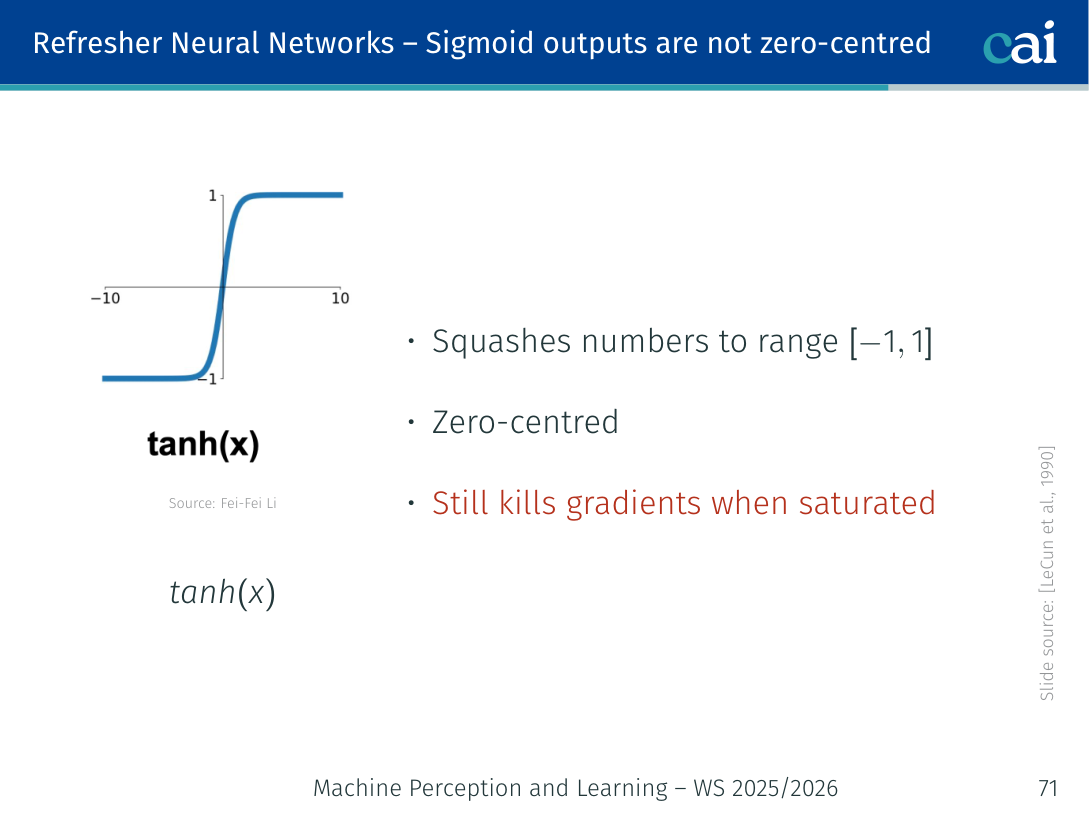
Tanh is zero-centered, but it still has the same saturation problems as sigmoid.

$\tanh (x)=\frac{e^x-e^{-x}}{e^x+e^{-x}}$

• Squashes numbers to $[-1,1]$ → zero-centred ✓
• Still kills gradients when saturated ✗
• Preferred over sigmoid in hidden layers, but ReLU is better

ReLU

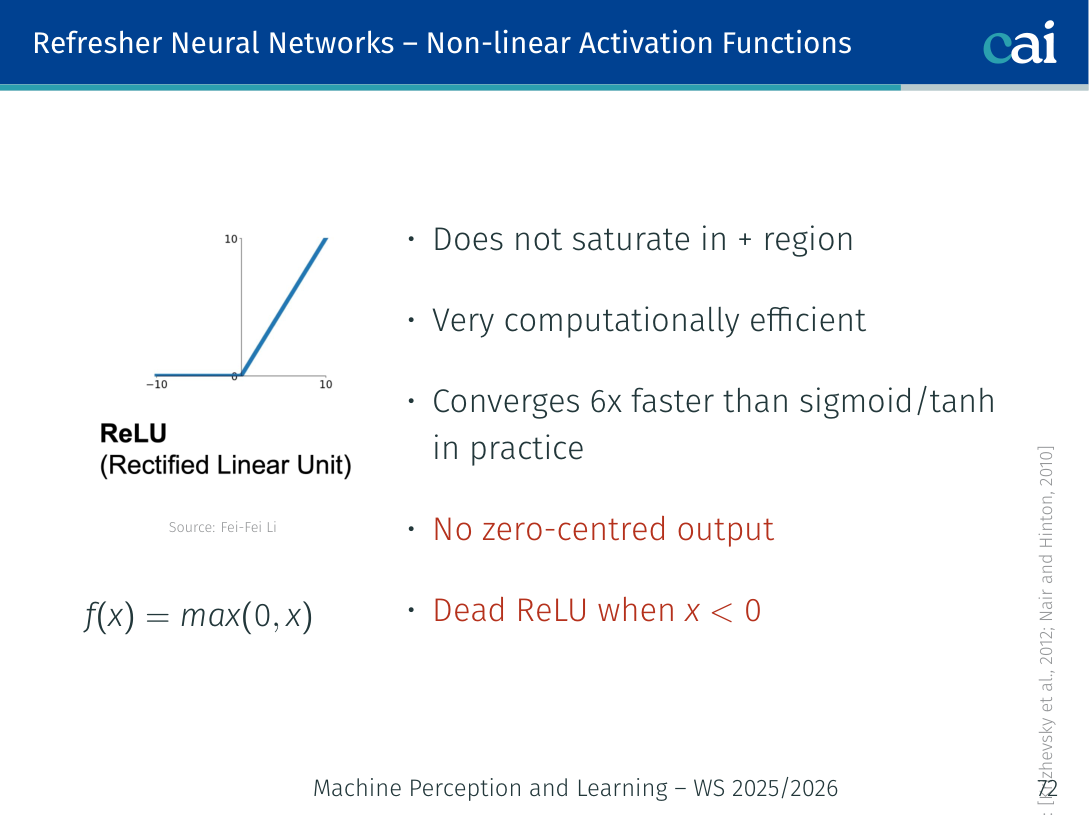
ReLU is fast and efficient, but watch out for "dead" neurons that stop learning.

$f(x)=\max (0,x)$

(Krizhevsky et al., 2012; Nair and Hinton, 2010)

Property	Value
Saturates in + region?	No ✓
Computationally efficient?	Yes ✓
Converges faster than sigmoid/tanh?	~6× faster ✓
Zero-centred output?	No ✗
Dead neurons?	Yes — a ReLU unit can permanently output 0 if it never activates ✗

Fix for dead ReLU: initialise ReLU neurons with slightly positive biases (e.g. 0.01).

Leaky ReLU / PReLU

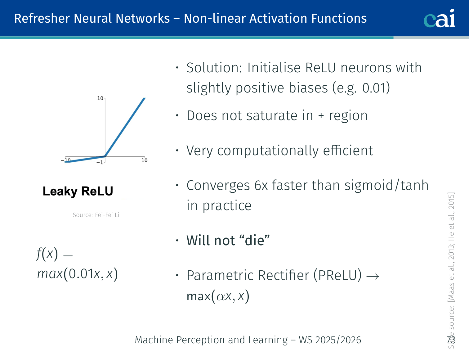
Leaky ReLU keeps a small slope for negative values so neurons never truly die.

$f(x)=\max (0.01x,x)$

(Maas et al., 2013; He et al., 2015)

• All benefits of ReLU ✓
• Does not saturate in the negative region → will not “die” ✓
• Parametric Rectifier (PReLU): replace the fixed $0.01$ slope with a learnable parameter $\alpha$: $\max (\alpha x,x)$

ELU (Exponential Linear Unit)

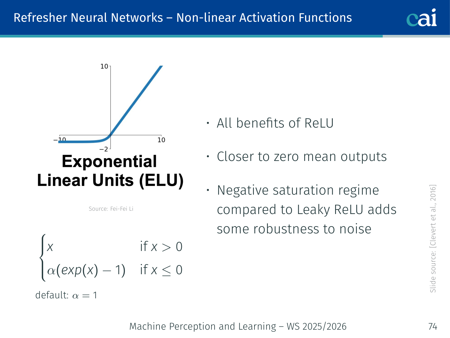
ELU gives you the best of ReLU but with smoother activations for negative inputs.

$f(x)=\{\begin{array}{ll}x& \text{if }x>0\\ \alpha (e^x-1)& \text{if }x\le 0\end{array}(\text{default: }\alpha =1)$

(Clevert et al., 2016)

• All benefits of ReLU ✓
• Closer to zero-mean outputs compared to Leaky ReLU ✓
• Negative saturation adds some robustness to noise ✓
• Computation requires exp() ✗

Maxout

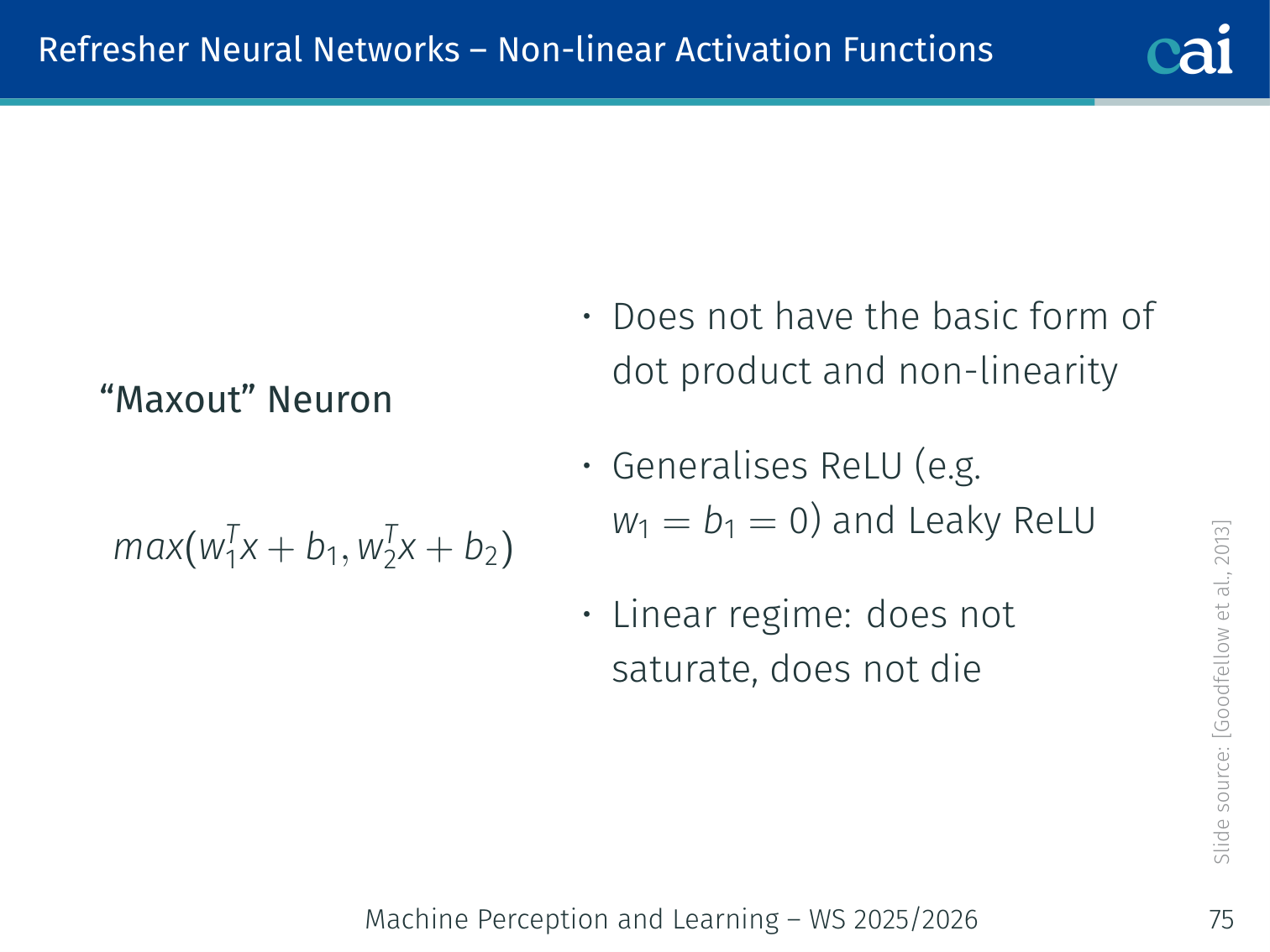
Maxout picks the best of several linear functions to create flexible activation shapes.

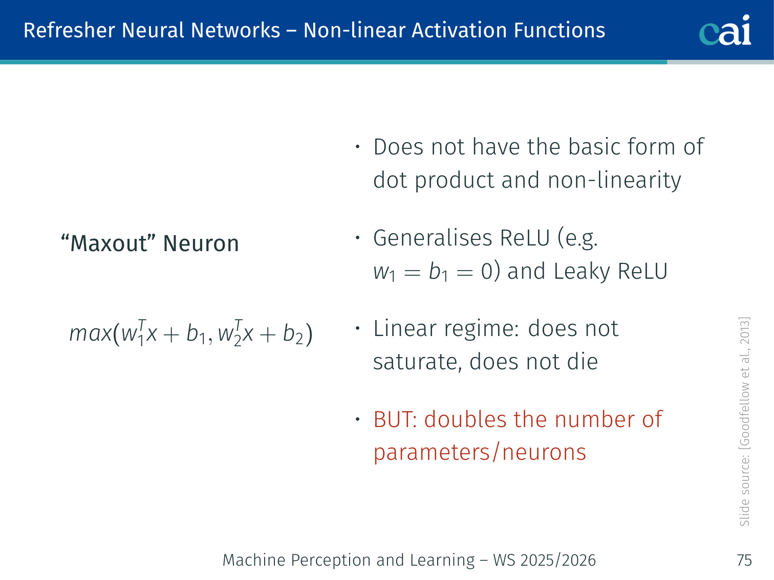
Another way to see Maxout: it's piecewise-linear and never saturates.

$f(x)=\max (w_1^{\top }x+b_1,w_2^{\top }x+b_2)$

(Goodfellow et al., 2013)

• Generalises ReLU (set $w_1=b_1=0$) and Leaky ReLU
• Linear regime: does not saturate, does not die ✓
• Does not have the basic dot-product + non-linearity form → doubles the number of parameters ✗

In Practice (TLDR)

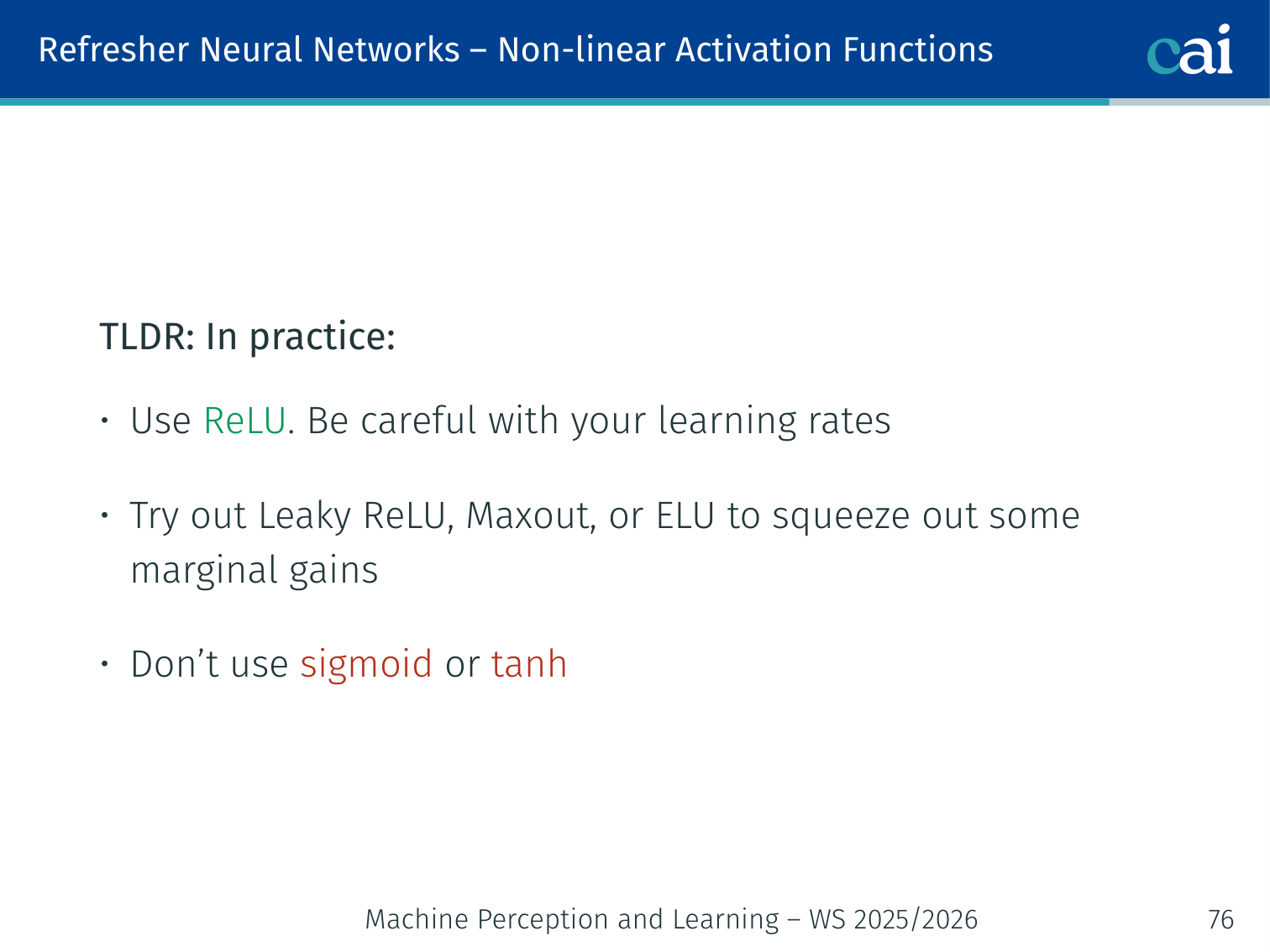
Some quick advice on which activation functions to use in practice.

• Use ReLU. Be careful with your learning rates.
• Try Leaky ReLU, Maxout, or ELU to squeeze out marginal gains.
• Don’t use sigmoid or tanh in hidden layers.

---

Weight Initialisation

All-Zero / Constant Init

Initializing everyone to the same value causes "symmetry" and breaks learning.

If all weights are the same value, all neurons compute identical gradients → they all update identically → the network never differentiates. This is the symmetry problem.

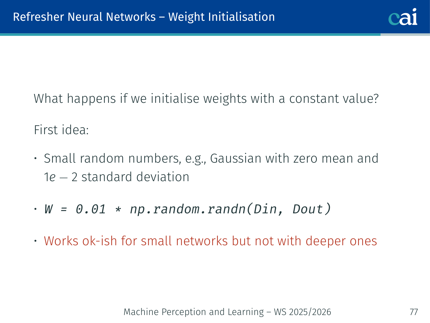
Small Random Numbers — W = 0.01 * randn(Din, Dout)

Tiny initial weights can make the signal fade away as it goes deeper.

Works okay for small networks, but not for deep ones:

• Activations tend to zero in deeper layers
• Gradients $\frac{\partial L}{\partial W}\to 0$ → no learning

Larger Random Numbers — W = 0.05 * randn(Din, Dout) (with tanh)

Large initial weights will saturate your activations and stall the training.

• Almost all neurons/activations saturate (outputs ≈ ±1)
• Gradients are again ≈ 0 → no learning

Xavier / Glorot Initialisation (2010)

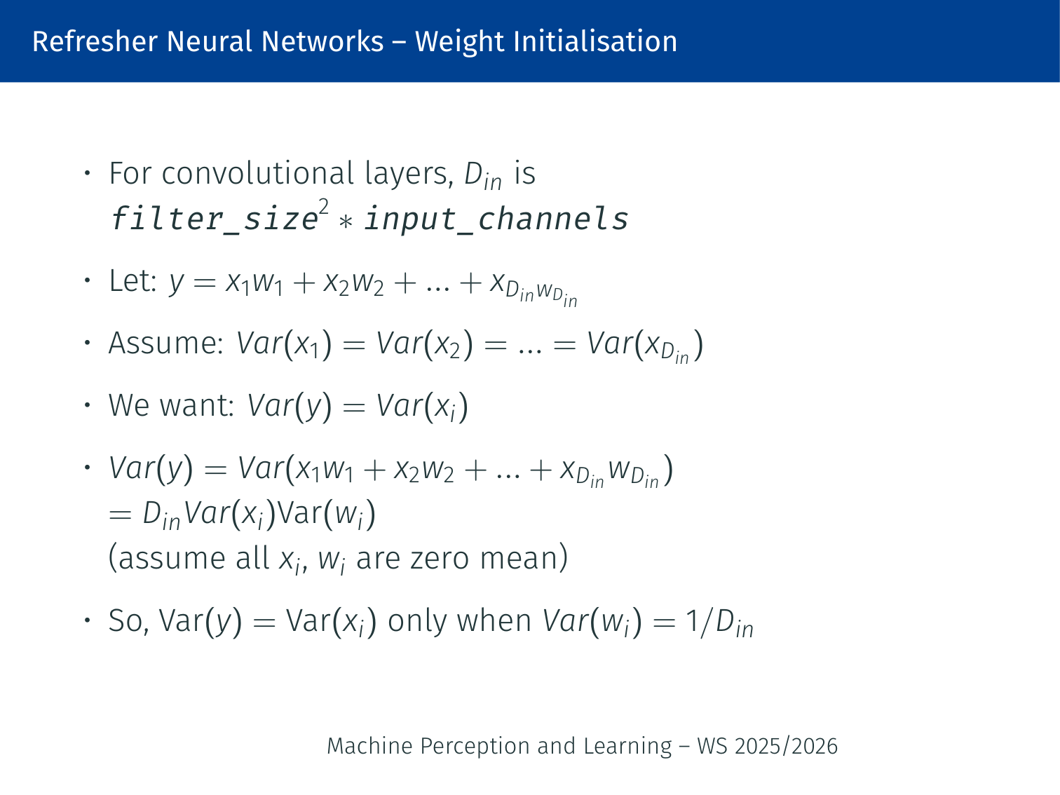
Xavier initialization keeps the signal steady as it passes through the network.

$\text{std}=\frac{1}{\sqrt{D_{\text{in}}}}$

Derivation: let $y={\sum }_{j=1}^{D_{\text{in}}}{x}_j{w}_j$. We want $\text{Var}(y)=\text{Var}(x_i)$.

Assuming all $x_i$ and $w_j$ are i.i.d. and zero-mean:

$\text{Var}(y)=D_{\text{in}}\cdot \text{Var}(x_i)\cdot \text{Var}(w_i)$

Setting $\text{Var}(y)=\text{Var}(x_i)$ gives $\text{Var}(w_i)=\frac{1}{D_{\text{in}}}$.

Activations are nicely scaled across all layers. Assumes a zero-centred activation function (e.g. tanh).

Kaiming / MSRA Initialisation — for ReLU (He et al., 2015)

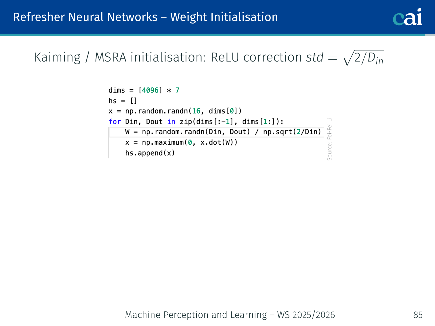
Kaiming initialization is the go-to choice when you’re using ReLU.

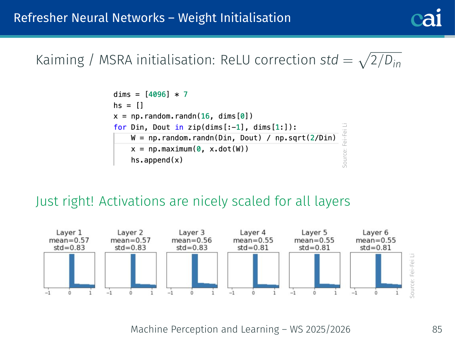
How Kaiming scaling keeps activations stable when half of them are zeroed out.

$\text{std}=\sqrt{\frac{2}{D_{\text{in}}}}$

Xavier breaks down for ReLU because ReLU is not zero-centred (it zeros out half the inputs). The factor of 2 compensates for the half that ReLU kills. With Kaiming init, activations are nicely scaled for all layers.

For convolutional layers: $D_{\text{in}}={\text{filter\_size}}^2\times \text{input\_channels}$

---

Batch Normalisation

Batch Normalisation was introduced to make deep networks easier to optimise (Ioffe and Szegedy, 2015). The original motivation was to reduce internal covariate shift: as lower layers change during training, the distribution seen by higher layers also changes. In practice, BatchNorm also makes training less sensitive to weight initialisation and typically stabilises optimisation.

BatchNorm Formula

For a mini-batch $B=\{x_1,\dots ,x_m\}$, BatchNorm computes

$${\mu }_B=\frac{1}{m}\sum _{i=1}^m{x}_i\text{and}{\sigma }_B^2=\frac{1}{m}\sum _{i=1}^m(x_i-{\mu }_B{)}^2$$

then normalises each activation:

$${\hat{x}}_i=\frac{x_i-{\mu }_B}{\sqrt{{\sigma }_B^2+\epsilon }}$$

and finally applies a learnable scale and shift:

$$y_i=\gamma {\hat{x}}_i+\beta$$

The parameters $\gamma$ and $\beta$ are learned, so the network can recover any useful mean or variance if needed.

Train Time vs. Test Time

Phase	Statistics used	Behaviour
Training	Mean/variance of the current mini-batch	Adds some noise, which can act as mild regularisation
Inference	Running mean/variance accumulated during training	Deterministic behaviour

For convolutional layers, BatchNorm is usually applied per channel, averaging over batch and spatial dimensions.

Why Does It Help?

BatchNorm often helps because it:

• makes the loss landscape smoother
• allows higher learning rates
• reduces sensitivity to poor initialisation
• improves gradient flow in deeper networks

Example: A deep CNN that becomes unstable with a large learning rate can often train cleanly once each Conv layer is followed by BatchNorm.

PyTorch Example

import torch.nn as nn
 
block = nn.Sequential(
    nn.Conv2d(3, 64, kernel_size=3, padding=1, bias=False),
    nn.BatchNorm2d(64),
    nn.ReLU(inplace=True),
    nn.MaxPool2d(2),
)

A common pattern is:

$$\text{Conv}\to \text{BatchNorm}\to \text{ReLU}$$

---

Regularisation

Why Regularise?

A model overfits when it fits the training data too closely, including noise and accidental patterns, but fails to generalise to unseen data. This is the classic bias-variance tradeoff:

• High bias: model is too simple → underfitting
• High variance: model is too flexible → overfitting

Regularisation adds constraints or noise so that the learned model generalises better.

L2 Regularisation / Weight Decay

L2 regularisation adds a penalty on large weights:

$${\mathcal{L}}_{\text{total}}={\mathcal{L}}_{\text{data}}+\lambda \Vert W{\Vert }_2^2$$

This encourages weights to stay small and smooths the fitted function. In deep learning, L2 regularisation is usually implemented as weight decay in the optimiser.

L1 Regularisation

L1 regularisation uses

$${\mathcal{L}}_{\text{total}}={\mathcal{L}}_{\text{data}}+\lambda \Vert W{\Vert }_1$$

Unlike L2, L1 encourages many weights to become exactly zero, so it tends to produce sparser models.

PyTorch: Weight Decay and Early Stopping

# 1. Weight Decay (L2 Regularization)
# Added directly as a parameter in the optimizer.
# This penalizes large weight values to improve generalization.
optimizer = torch.optim.Adam(model.parameters(), lr=0.01, weight_decay=1e-3)

Explanation:

• weight_decay: In PyTorch optimizers, this parameter implements L2 Regularization by adding a penalty proportional to the squared magnitude of weights to the loss, preventing them from growing too large.
• Early Stopping: A heuristic that stops training when validation performance stops improving for a fixed number of epochs (patience).

Dropout

Dropout randomly zeros activations during training (Srivastava et al., 2014). If $h$ is a hidden representation and $m_i\sim \text{Bernoulli}(1-p)$, then

$$\tilde{h}=m\odot h$$

where $p$ is the dropout rate.

Intuition:

• each mini-batch sees a slightly different sub-network
• neurons cannot rely too strongly on any single other neuron
• this reduces co-adaptation and improves generalisation

Classically, activations are scaled at test time by $(1-p)$. In modern libraries such as PyTorch, inverted dropout is used instead: activations are scaled during training, so evaluation needs no extra rescaling.

Data Augmentation

Data augmentation is another form of regularisation: random crops, flips, colour jitter, noise, etc. It does not directly penalise the weights, but it makes the learning problem harder to overfit.

Summary of Common Regularisers

Method	Main effect	Typical outcome
L2 / weight decay	Penalises large weights	Smoother, more stable models
L1	Encourages sparsity	Many weights become zero
Dropout	Randomly removes activations during training	More robust hidden representations
Data augmentation	Increases effective data diversity	Better generalisation to new samples

Example: If training accuracy keeps rising but validation accuracy stalls, adding weight decay and dropout is often a good first fix before changing the architecture.

Practical Guidance

A good default recipe is:

• weight decay for most models
• dropout in fully connected heads or smaller datasets
• data augmentation for vision tasks

In practice, weight decay + dropout is a strong baseline regularisation combination.

PyTorch Implementation: Multi-Layer Perceptron (MLP)

A straightforward way to build an MLP using PyTorch.

Below is a practical implementation of a simple MLP in PyTorch.

import torch
import torch.nn as nn
 
# 1. Define the MLP Architecture
# All PyTorch models must inherit from nn.Module
class MLP(nn.Module):
    def __init__(self, n_inputs=1):
        super().__init__()
        # nn.Sequential executes layers in the order they are added
        self.net = nn.Sequential(
            # Linear layer: computes out = x * weight^T + bias
            # Maps input features to 10 hidden features
            nn.Linear(n_inputs, 10),
 
            # Tanh activation function provides non-linearity
            nn.Tanh(),
 
            # Output layer: maps 10 hidden features back to 1 output
            nn.Linear(10, 1),
        )
 
    def forward(self, x):
        # Defines the computation performed at every call
        return self.net(x)
 
# 2. Setup Training
model = MLP()
# Adam is an adaptive optimizer; lr is the learning rate
optimizer = torch.optim.Adam(model.parameters(), lr=0.01)
# MSELoss (Mean Squared Error) is the standard loss for regression
criterion = nn.MSELoss()
 
# 3. Training Loop
model.train() # Set the model to training mode
for epoch in range(200):
    # STEP 1: Clear existing gradients from the last step
    optimizer.zero_grad()
 
    # STEP 2: Forward pass - get model predictions
    outputs = model(x)
 
    # STEP 3: Compute the loss (error)
    loss = criterion(outputs, targets)
 
    # STEP 4: Backpropagation - calculate gradients for all parameters
    loss.backward()
 
    # STEP 5: Optimization - update weights based on gradients
    optimizer.step()

Key PyTorch Concepts:

• nn.Module: The base class for all neural network modules. Your model must inherit from it to utilize PyTorch’s parameter tracking.
• nn.Sequential: A container that wraps layers in a sequence, automatically passing the output of one to the next.
• forward(): Defines the computation performed at every call. You don’t call this directly; use model(x).
• optimizer.zero_grad(): Crucial step to clear gradients from the previous iteration; otherwise, they accumulate across batches.
• loss.backward(): Triggers Autograd to compute the gradient of the loss with respect to all model parameters using the chain rule.

Logistic Regression (Scikit-Learn)

While not PyTorch, Scikit-Learn is the industry standard for traditional ML baselines.

from sklearn.linear_model import LogisticRegression
 
# 1. Create the Model
# max_iter is the limit on solver iterations for convergence
model = LogisticRegression(max_iter=1000)
 
# 2. Train the Model (fit to data)
# X_train: features, y_train: labels
model.fit(X_train, y_train)
 
# 3. Evaluate Performance
# returns the mean accuracy on the test data
accuracy = model.score(X_test, y_test)

Concepts:

• fit(): The standard Scikit-Learn method for training a model on data.
• score(): Returns the mean accuracy on the given test data and labels.

---

Summary

1. ML = automatically learning from data without explicit programming
2. Neural nets = stacked linear transformations + non-linearities
3. Optimisation = minimise the loss via gradient descent
4. Backpropagation = efficient gradient computation via the chain rule through computational graphs
5. Activation functions: use ReLU (avoid sigmoid/tanh in hidden layers)
6. Weight initialisation: Xavier for tanh networks, Kaiming for ReLU networks
7. BatchNorm normalises activations and makes optimisation more stable
8. Regularisation improves generalisation; strong defaults are weight decay + dropout

---

References

• Ioffe, Szegedy (2015) — Batch normalization: Accelerating deep network training by reducing internal covariate shift. ICML.
• Srivastava, Hinton, Krizhevsky, Sutskever, Salakhutdinov (2014) — Dropout: A simple way to prevent neural networks from overfitting. JMLR, 15:1929–1958.

Applied Exam Focus

• Loss Functions: Use MSE for regression and Cross-Entropy for classification. Cross-Entropy penalizes confident wrong answers more heavily.
• Activation Choice: Default to ReLU for hidden layers. Avoid Sigmoid/Tanh in deep networks due to the vanishing gradient problem (gradients $\approx 0$ when saturated).
• Initialization: Always use Kaiming (He) initialization when using ReLU to keep the variance of activations stable across layers.

---

Back to MPL Index | Next: (y-02) CNNs | (y) Return to Notes | (y) Return to Home