L02 — Convolutional Neural Networks

Previous: L01 — Intro | Back to MPL Index | Next: (y-03) Vision CNNs

Mental Model First

CNNs work because images have local structure: nearby pixels matter together, and the same kinds of patterns can appear in many locations.
A convolution filter is a small reusable detector that scans the image for a pattern such as an edge, corner, or texture.
Pooling and depth gradually trade exact location for stronger semantic meaning: edges become motifs, motifs become parts, and parts become objects.
If one question guides this lecture, let it be: how can we recognise visual patterns without relearning the same detector at every pixel location?

Human Visual Perception

The Human Eye

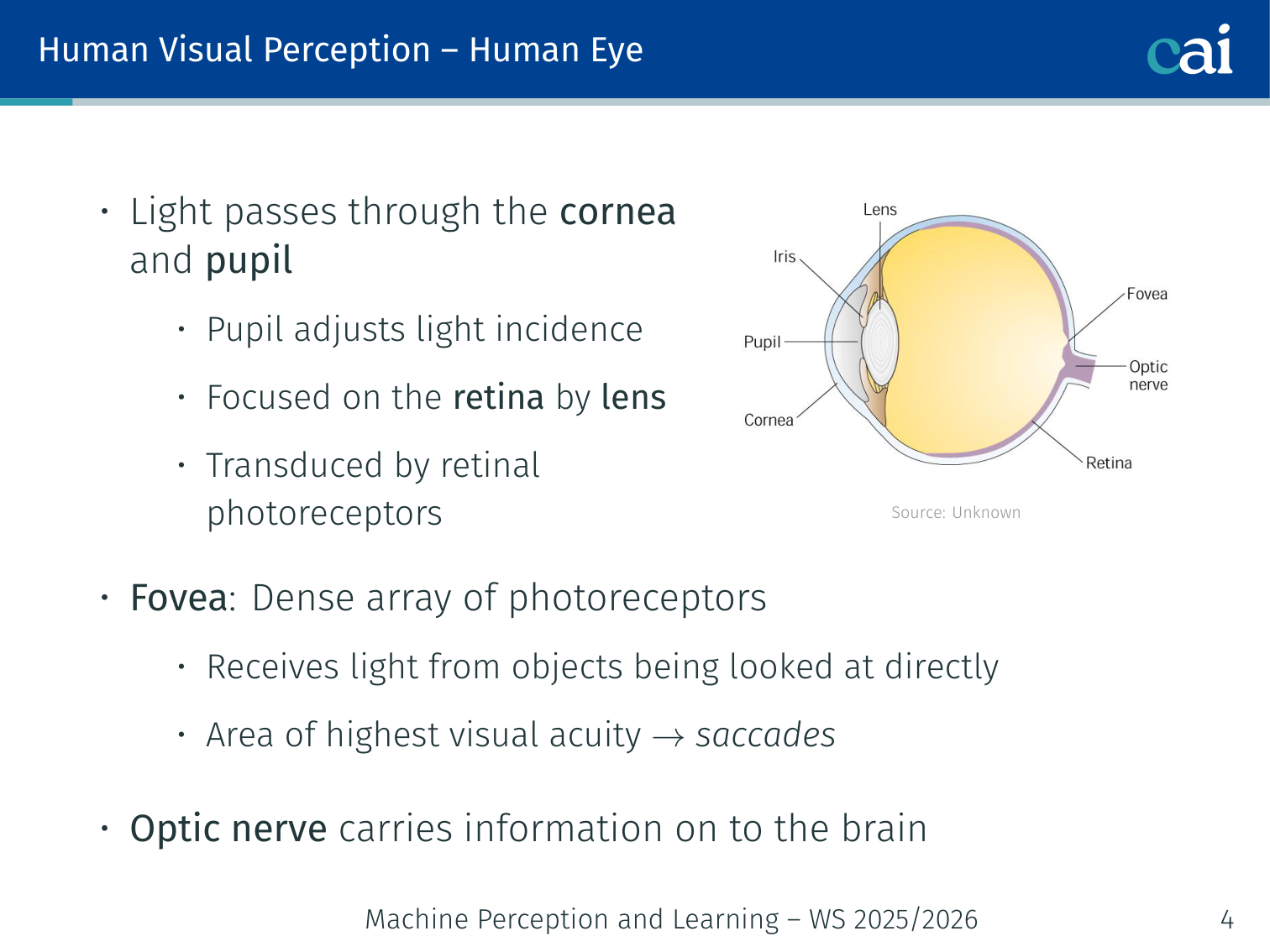
A quick look at how the human eye is wired, from the retina to the photoreceptors.

Light passes through the cornea and pupil
The pupil adjusts light incidence; the lens focuses light onto the retina
The fovea: dense array of photoreceptors; receives light from objects looked at directly; area of highest visual acuity (hence saccades)
The optic nerve carries information from the retina on to the brain

Retina

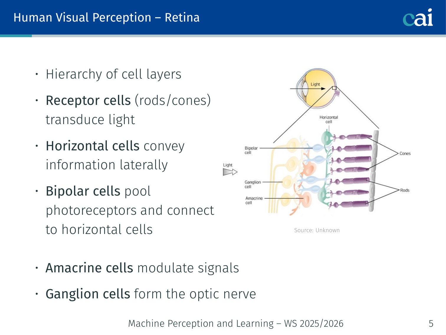
The layers of cells in our retina that start processing light before it even hits the brain.

Hierarchy of cell layers:

Receptor cells (rods/cones) transduce light
Horizontal cells convey information laterally
Bipolar cells pool photoreceptors and connect to horizontal cells
Amacrine cells modulate signals
Ganglion cells form the optic nerve

Cell Types

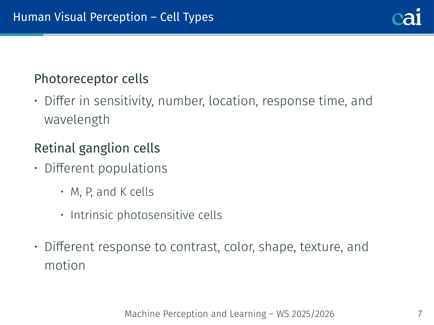
Comparing the different types of photoreceptor and ganglion cells in our eyes.

Photoreceptor cells differ in sensitivity, number, location, response time, and wavelength.

Retinal ganglion cells have different populations (M, P, and K cells; intrinsic photosensitive cells) with different responses to contrast, color, shape, texture, and motion.

Photoreceptors

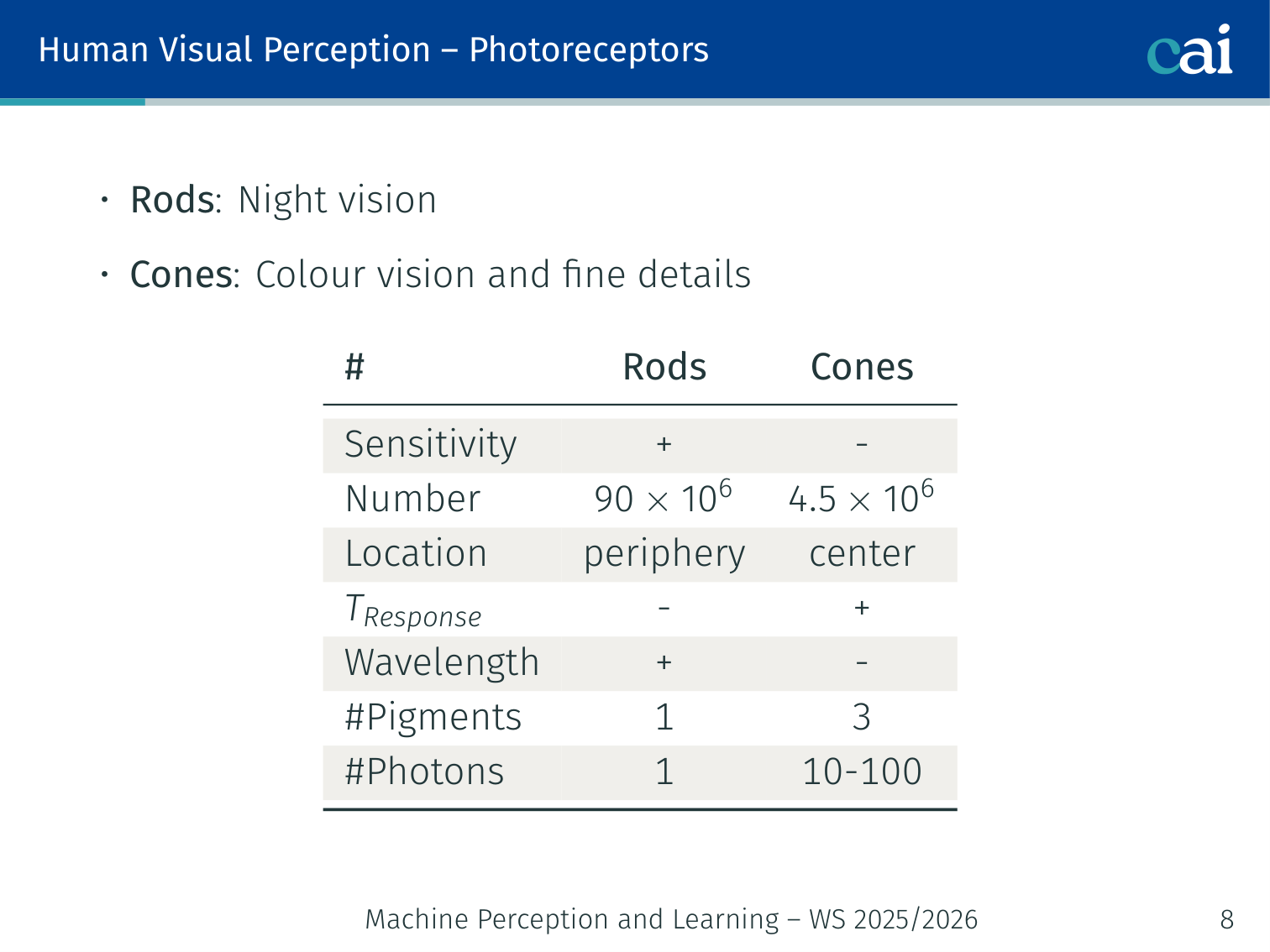
The key differences between rods and cones, like how they handle light and color.

	Rods	Cones
Sensitivity	+	−
Number	90 × 10⁶	4.5 × 10⁶
Location	periphery	center
Response time	−	+
Wavelength range	+	−
# Pigments	1	3
# Photons needed	1	10–100

Rods: night vision
Cones: colour vision and fine details

Thalamus and the LGN

The LGN acts like a relay station, sorting visual signals on their way to the cortex.

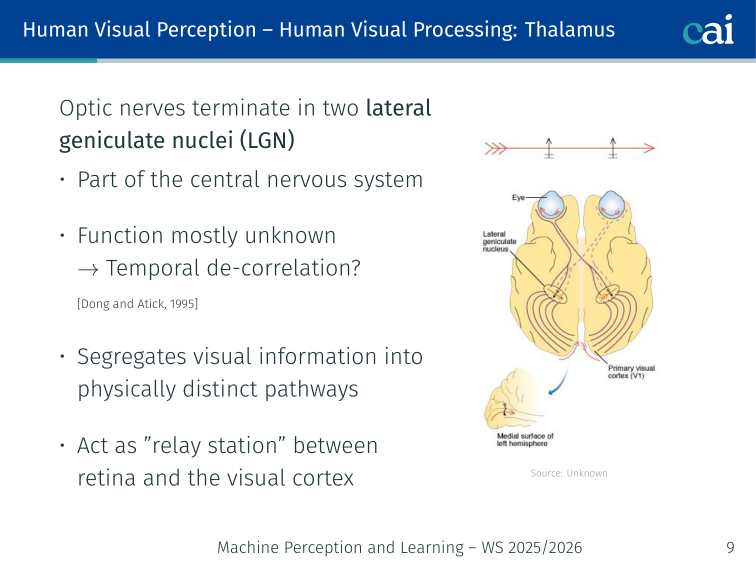
Optic nerves terminate in two lateral geniculate nuclei (LGN):

Part of the central nervous system; function mostly unknown → temporal de-correlation? [Dong and Atick, 1995]
Segregates visual information into physically distinct pathways
Acts as a “relay station” between retina and the visual cortex

Visual Cortex

The visual cortex is a hierarchy that starts with simple features in V1.

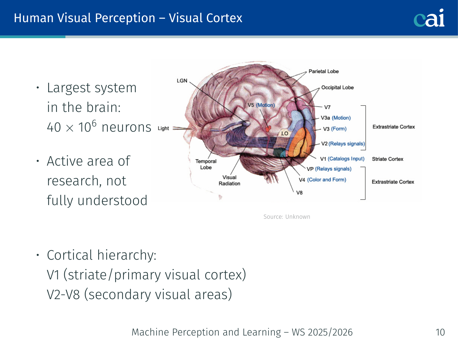
Largest system in the brain: 40 × 10⁶ neurons; active area of research, not fully understood
Cortical hierarchy: V1 (striate/primary visual cortex) → V2–V8 (secondary visual areas)

Two-Streams Hypothesis

The two main paths in the brain: one for "where" things are and one for "what" they are.

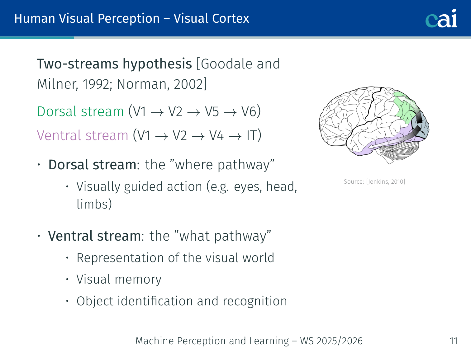
[Goodale and Milner, 1992; Norman, 2002]

Dorsal stream (V1 → V2 → V5 → V6): the “where pathway” — visually guided action (eyes, head, limbs)
Ventral stream (V1 → V2 → V4 → IT): the “what pathway” — representation of the visual world, visual memory, object identification and recognition

Specificity vs. Invariance

The constant tug-of-war between being specific enough to identify things and invariant enough to handle changes.

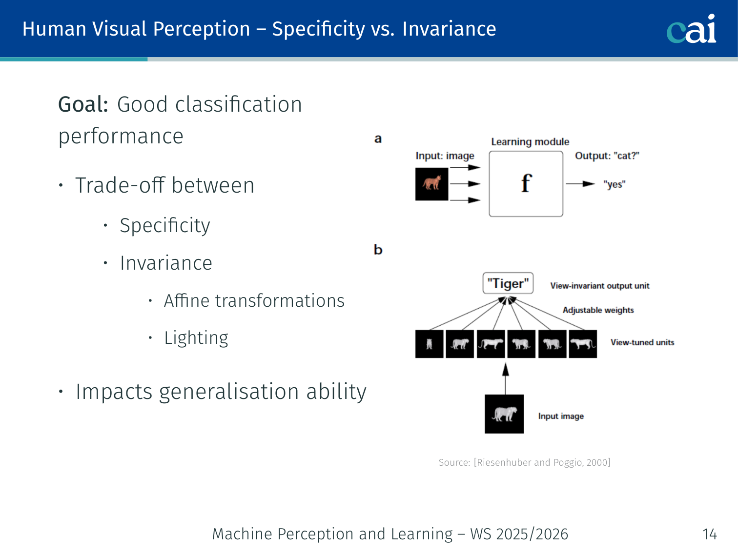
Goal: good classification performance requires a trade-off between:

Specificity — sensitivity to fine detail
Invariance — robustness to affine transformations and lighting changes

This trade-off directly impacts generalisation ability.

Simple and Complex Cells

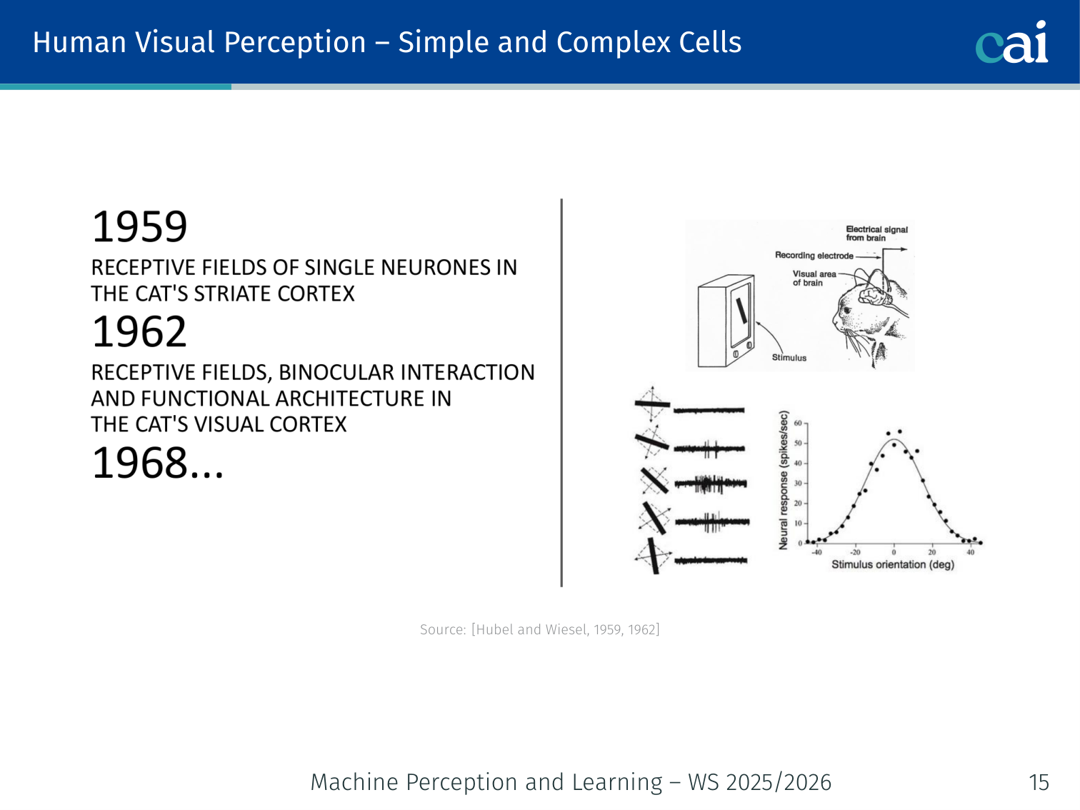
Simple cells care about exact location, while complex cells just want to see the right orientation.

[Hubel and Wiesel, 1959, 1962]

Simple cells: respond to oriented edges/bars at a specific location
Complex cells: respond to the same orientations regardless of exact location — position invariance

Receptive Field

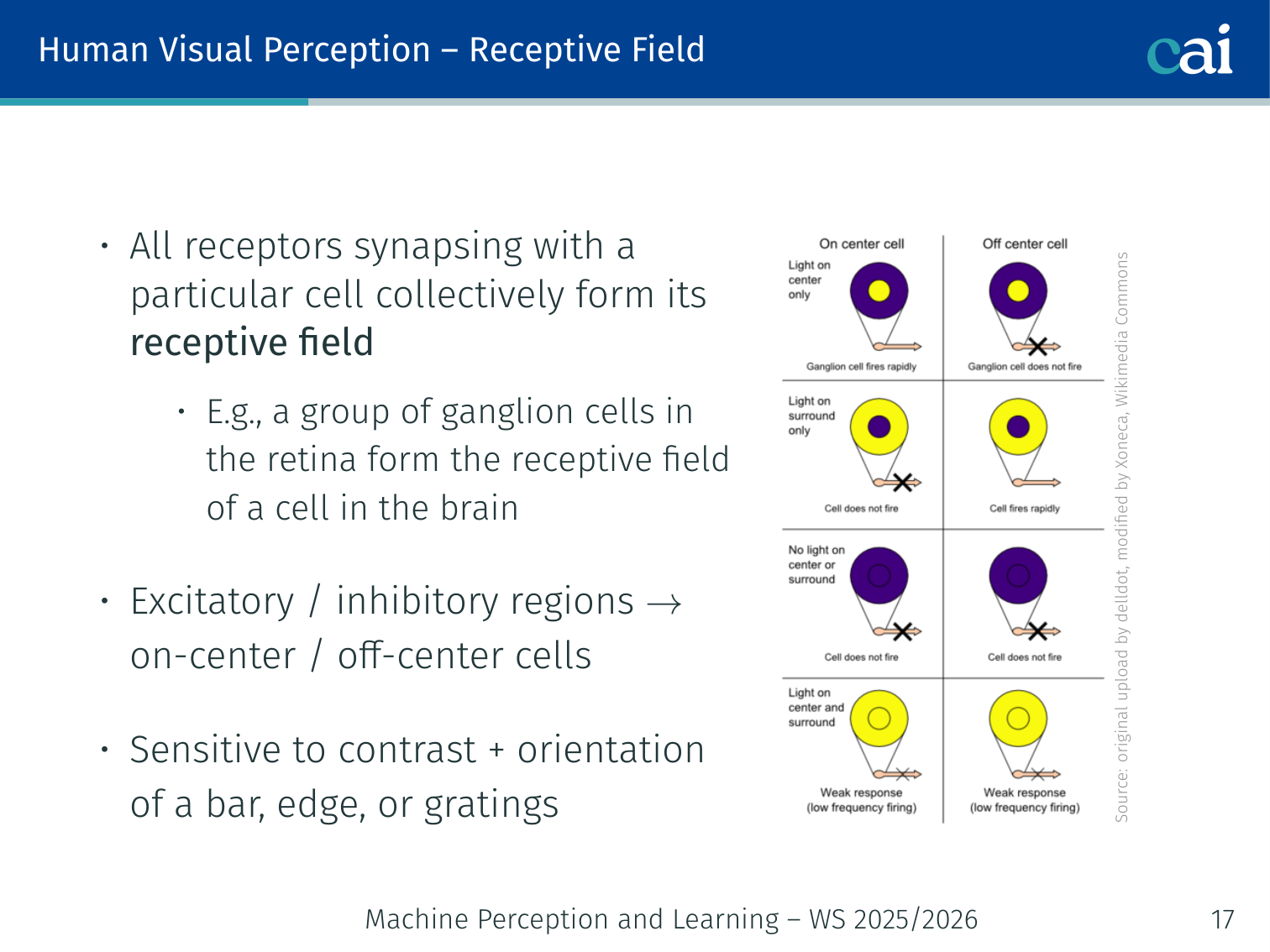
On-center and off-center fields show how our neurons react to contrast.

All receptors synapsing with a particular cell collectively form its receptive field
Cells have excitatory/inhibitory regions → on-center / off-center cells
Sensitive to contrast and orientation of a bar, edge, or gratings

Hierarchical Organisation

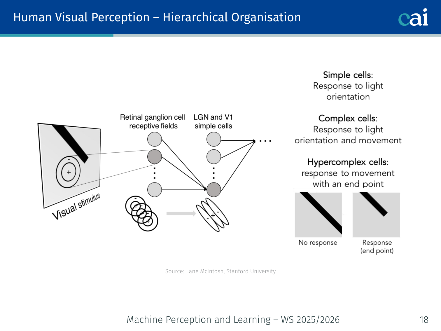
The visual system builds up from simple edges to full object descriptions.

The visual system builds progressively more complex representations from low-level edge detectors to higher-level object descriptions.

Invariance to Affine Transforms

How our brain recognizes objects even when they move, change size, or turn.

Neurons in the inferior temporal cortex show invariance to position, scale, and view [Logothetis et al., 1995] — a property that CNNs aim to replicate.

History of Deep Learning

HMAX Model

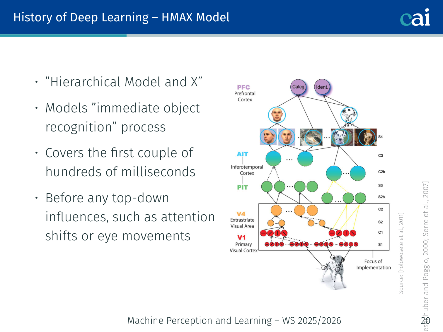
The HMAX model mimics the brain by switching between feature detection and pooling.

[Riesenhuber and Poggio, 2000; Serre et al., 2007]

Models the “immediate object recognition” process (first few hundred milliseconds — before top-down influences such as attention shifts or eye movements)
Alternates between S-units and C-units; many iterations allow construction of complex objects from low-level features

S-cell (simple cell) response — tuned to specific stimuli with typically small receptive fields:

$y = exp (- \frac{1}{2 σ ^{2}} \sum_{j = 1}^{n_{S_{k}}} (w_{j} - x_{j})^{2})$

$σ$ defines the sharpness of the bell-shaped tuning
$w$ are the trainable parameters

C-cell (complex cell) response — combines output from multiple S-units to increase invariance and receptive field:

$y = max_{j = 1 \dots n_{C_{k}}} x_{j}$

Response corresponds to the strongest of its afferents — a pooling operation

Neocognitron (1982)

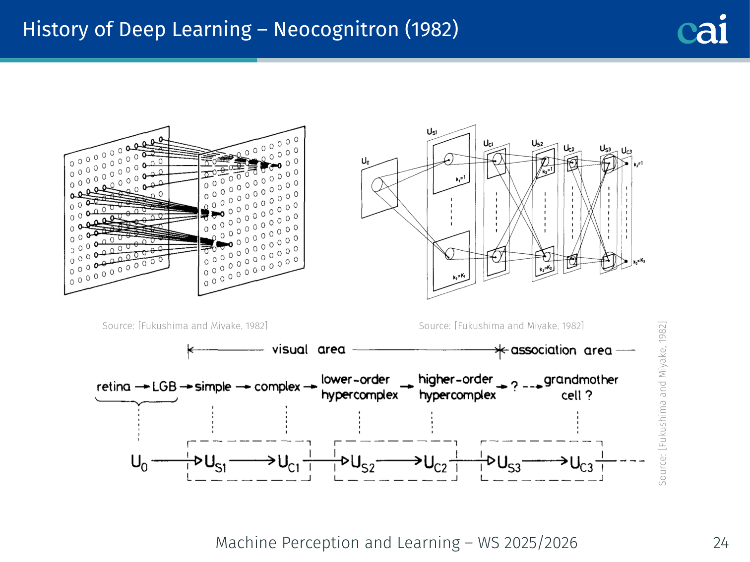
The Neocognitron was a huge early step towards the CNNs we use today.

[Fukushima and Miyake, 1982] — an early CNN-like architecture with alternating S-layers and C-layers, directly implementing the Hubel-Wiesel hierarchy.

LeNet-5 (1998)

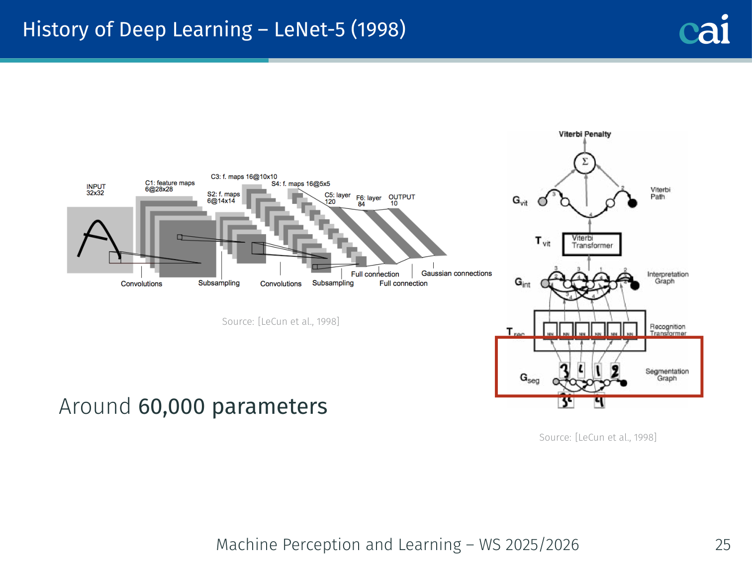
LeNet-5, the classic network that first mastered handwritten digit recognition.

[LeCun et al., 1998] — convolutional + pooling + fully-connected layers; ~60,000 parameters; trained on handwritten digit recognition.

AlexNet (2012)

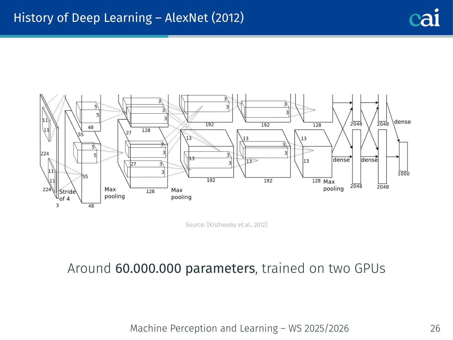
AlexNet is the model that really kicked off the deep learning revolution in 2012.

[Krizhevsky et al., 2012] — ~60,000,000 parameters, trained on two GPUs. Evaluated on the large-scale ImageNet dataset [Deng et al., 2009] and dramatically outperformed prior methods.

Fine-Grained Prediction

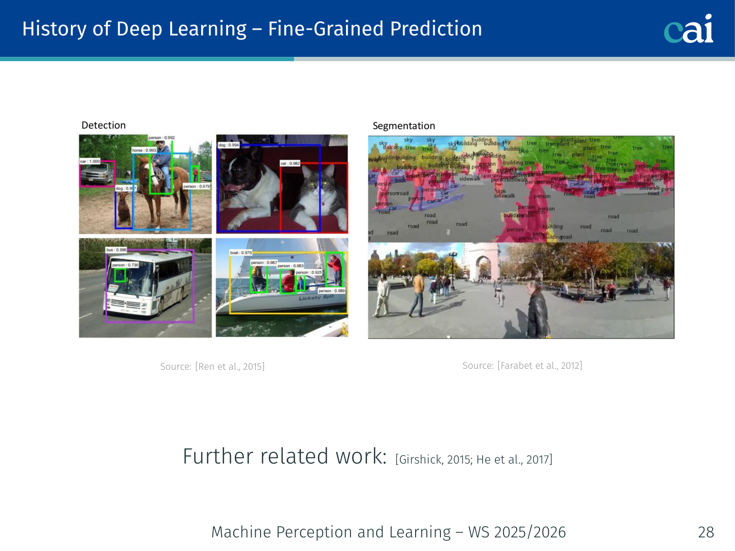
CNNs aren't just for classification; they're great for detection and labeling too.

Beyond classification, CNNs were extended to dense predictions — object detection [Ren et al., 2015; Girshick, 2015; He et al., 2017] and scene labelling [Farabet et al., 2012].

Deep Learning in a Nutshell

Traditional Approach

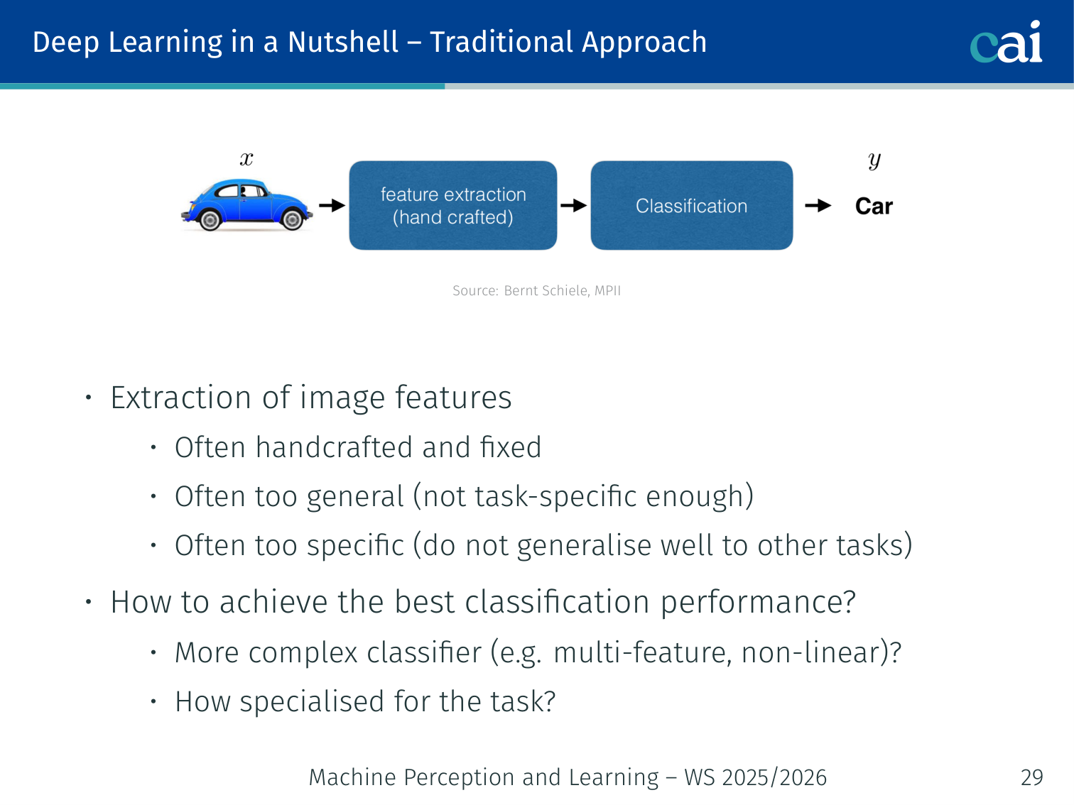
Before deep learning, we had to hand-craft every single visual feature.

Image features were often:

Handcrafted and fixed
Too general (not task-specific enough), or too specific (do not generalise well to other tasks)

Trainable Features

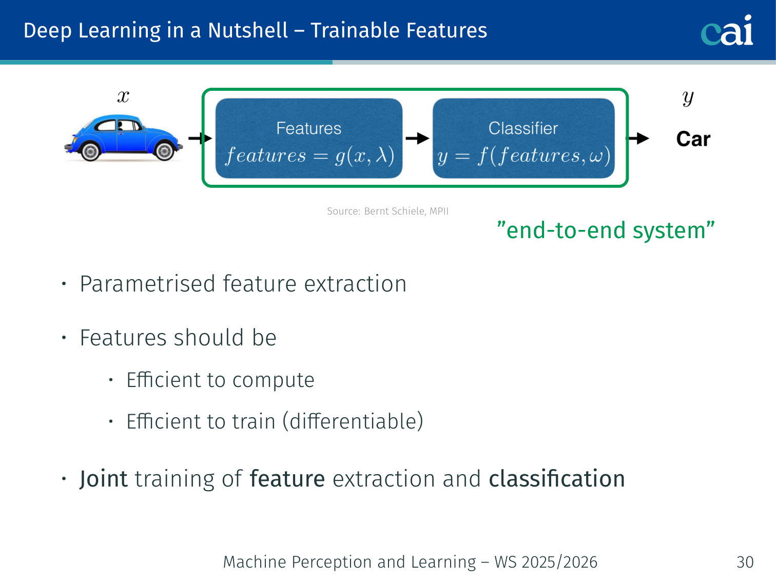
Nowadays, we let the network learn the best features directly from the data.

Parametrised feature extraction: features are learned, not hand-coded
Features should be efficient to compute and efficient to train (differentiable)
Joint training of feature extraction and classification → “end-to-end system”

Summary of Main Ideas

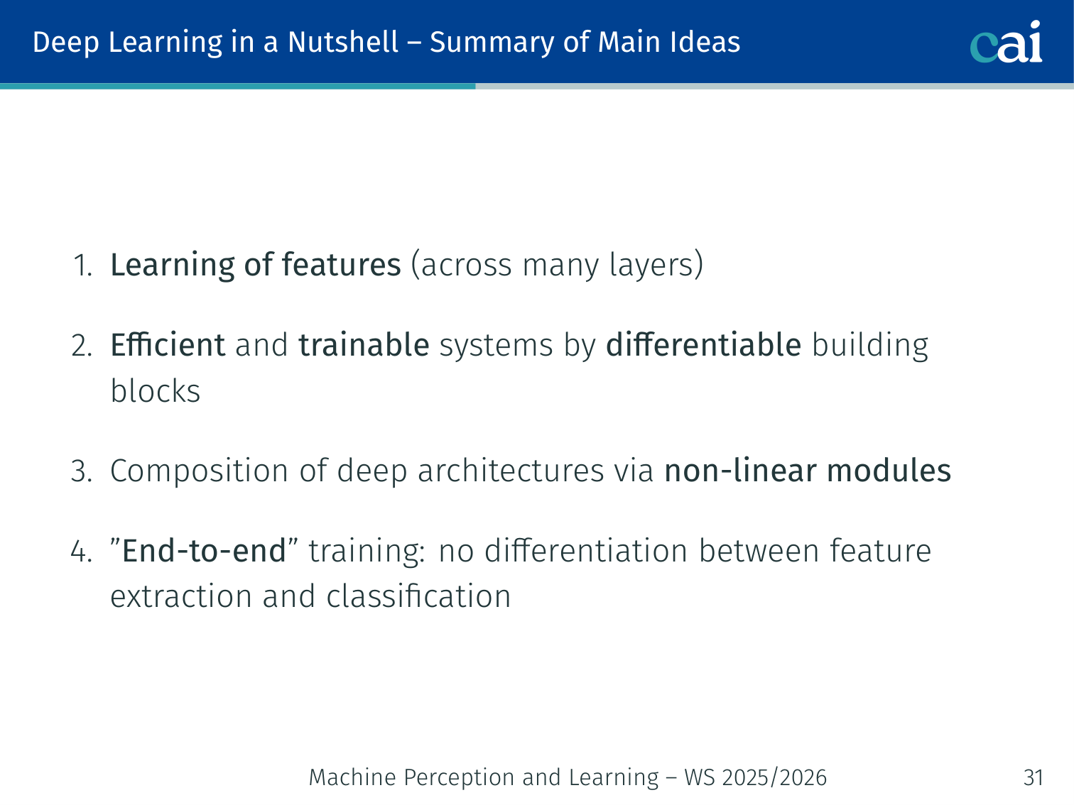
A quick wrap-up of the big ideas: hierarchies, differentiability, and end-to-end training.

Learning of features across many layers
Efficient and trainable systems via differentiable building blocks
Composition of deep architectures via non-linear modules
“End-to-end” training: no differentiation between feature extraction and classification

Convolutional Neural Networks

Fully Connected Layer

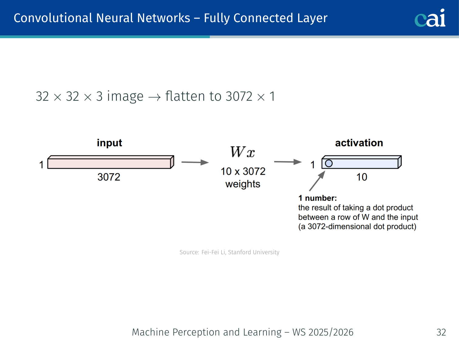
A fully connected layer treats an image like a flat list, losing all spatial info.

A 32×32×3 image flattened to 3072×1 is fed into a dense layer. This ignores all spatial structure and scales poorly.

Convolutional Layer

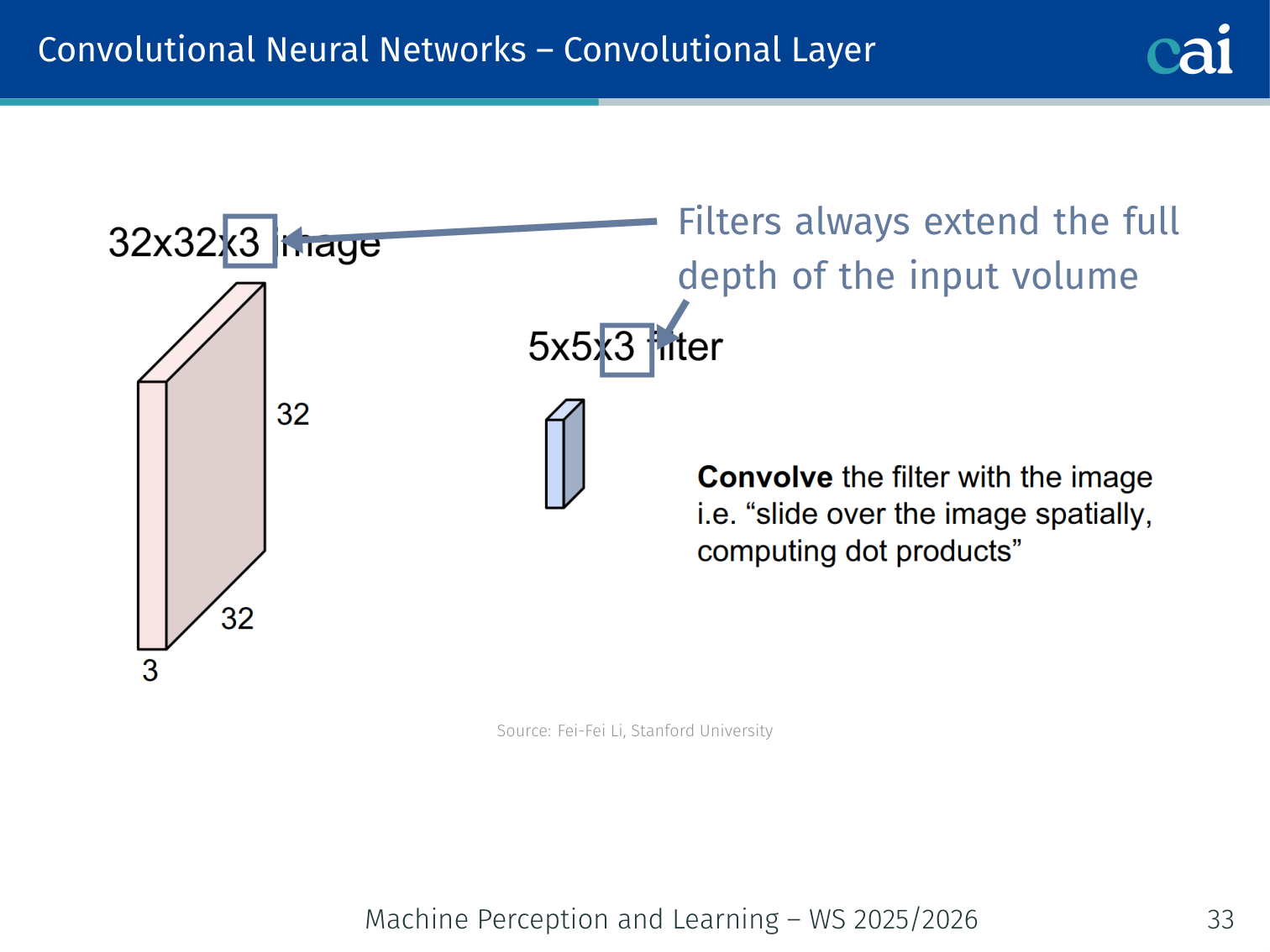
A convolution filter slides over the image to create a map of where it found a pattern.

A filter (kernel) slides across the spatial dimensions of the input
Filters always extend the full depth of the input volume
The filter computes a dot product at each spatial position → produces an activation map (also called a feature map)

💡 Example: The Sobel Filter (Edge Detection)

A CNN doesn’t “know” it’s looking at a cat. It first learns to find edges. One of the most famous examples is the Sobel Filter for finding vertical edges:

$K = - 1 - 2 - 1 000121$

If you slide this over a solid white area, the result is $0$ .
If you slide this over a vertical edge (white on left, black on right), the result is a large positive number.
If you slide this over a horizontal edge, the result is $0$ .

In a CNN, we don’t hard-code these numbers. The network learns them during training!

Multiple Activation Maps

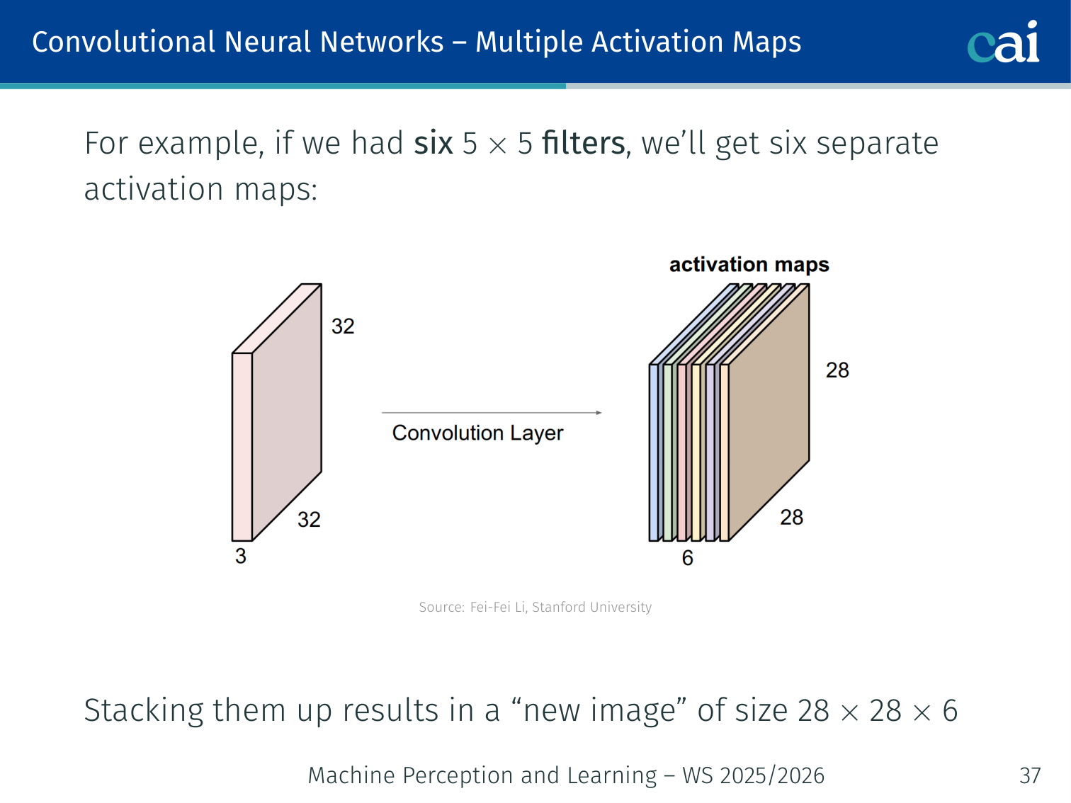
Stacking maps from different filters gives us a rich "volume" of features.

Using multiple filters in parallel produces multiple feature maps. For example, six 5×5 filters applied to a 32×32×3 input produce six separate activation maps of size 28×28, which stack into a volume of 28×28×6.

💡 Intuition: Convolution vs. Flattening (The “Face” Example)

Imagine you are looking for a face in a photo.

Fully Connected Approach (Flattening): You treat the photo like a giant list of numbers. To recognize a face, you have to learn what a face looks like at every single possible pixel location. If the face moves one pixel to the left, the whole list of numbers changes, and the network might not recognize it anymore.
Convolutional Approach: You use a small “Face Detector” (the filter) and slide it across the image. The detector only cares what a face looks like locally. If it finds a face anywhere, it shouts “Found one!“. This makes the network much more efficient and robust.

🧠 Deep Dive: Translation Invariance

One of the biggest strengths of CNNs is Translation Invariance (or Equivariance).

How it works:

Weight Sharing: Because the same filter is used everywhere, if an edge exists in the top-left or bottom-right, the same weights will detect it.
Pooling: Max pooling takes a small region (e.g., 2x2) and picks the strongest signal. If a feature moves slightly within that 2x2 area, the output of the pooling layer stays exactly the same.

This is why a CNN can recognize a “cat” regardless of whether the cat is in the corner of the image or right in the middle.

Key Idea

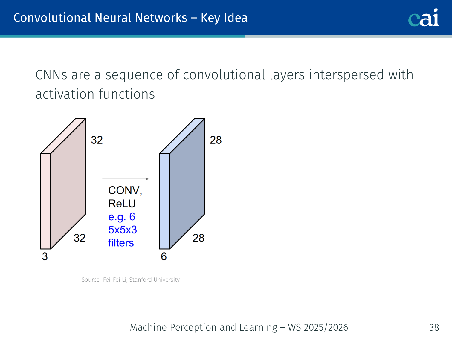
The core of a CNN is just a sequence of convolutions and activations.

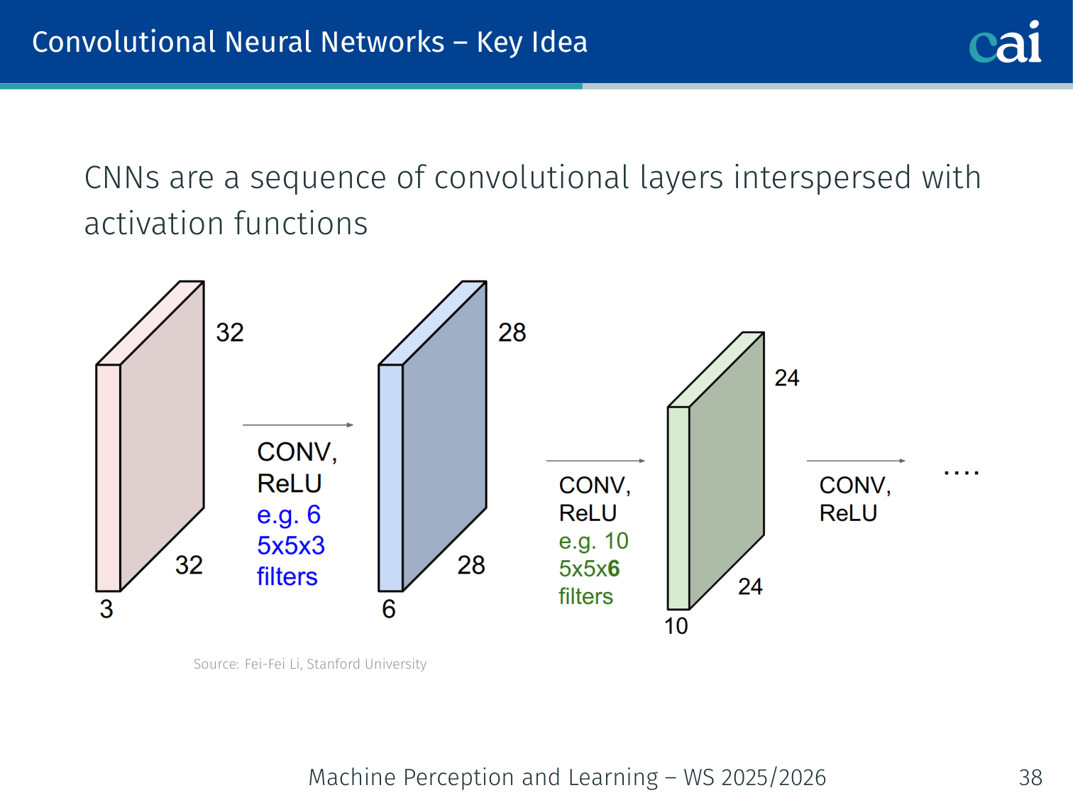
As we go deeper, the representations become more abstract and meaningful.

CNNs are a sequence of convolutional layers interspersed with activation functions. Each layer learns increasingly abstract representations.

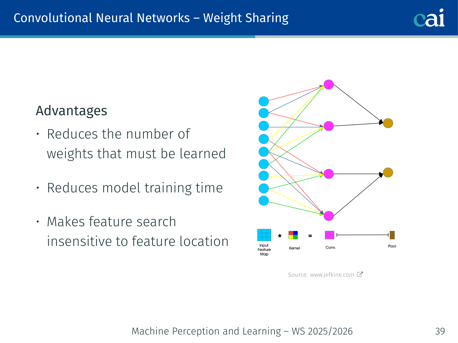
Weight sharing means the same filter works everywhere, which is super efficient.

The same filter weights are applied at every spatial position. Advantages:

Reduces the number of weights that must be learned
Reduces model training time
Makes feature search insensitive to feature location

🧠 Deep Dive: Why Many Small Filters Beat One Large Filter

One design choice that became very influential was using mostly 3x3 filters instead of a few very large kernels.

A single 7x7 convolution sees a large area in one step, but it has many parameters.
Three stacked 3x3 convolutions produce a similar effective receptive field while inserting non-linearities between the layers.
Those extra non-linearities let the network learn more complex functions than one large linear filter could.

Parameter count makes this concrete:

One 7x7 filter over $C$ channels needs $49 C$ weights per output channel.
Three 3x3 filters need $27 C$ weights per output channel in the simplest comparison.

So stacking small filters is not only cheaper, it also gives the model more depth, more expressiveness, and better gradient flow.

Visualisation

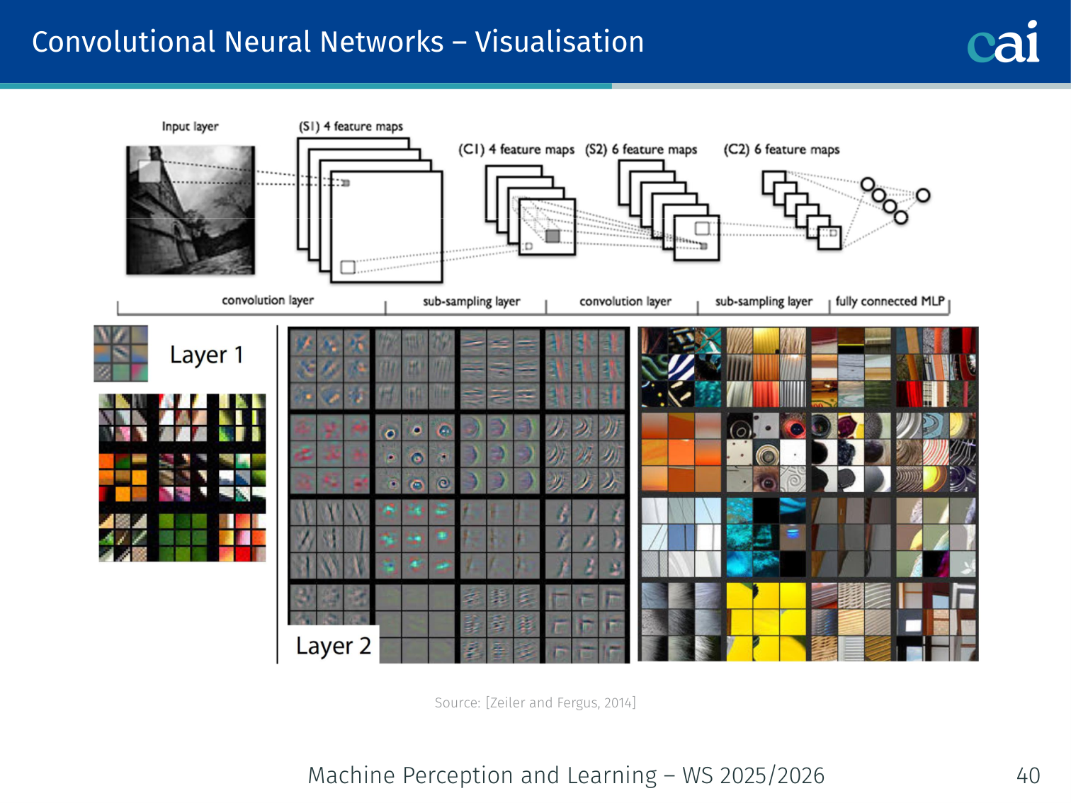
Early layers mostly look for simple things like edges and colors.

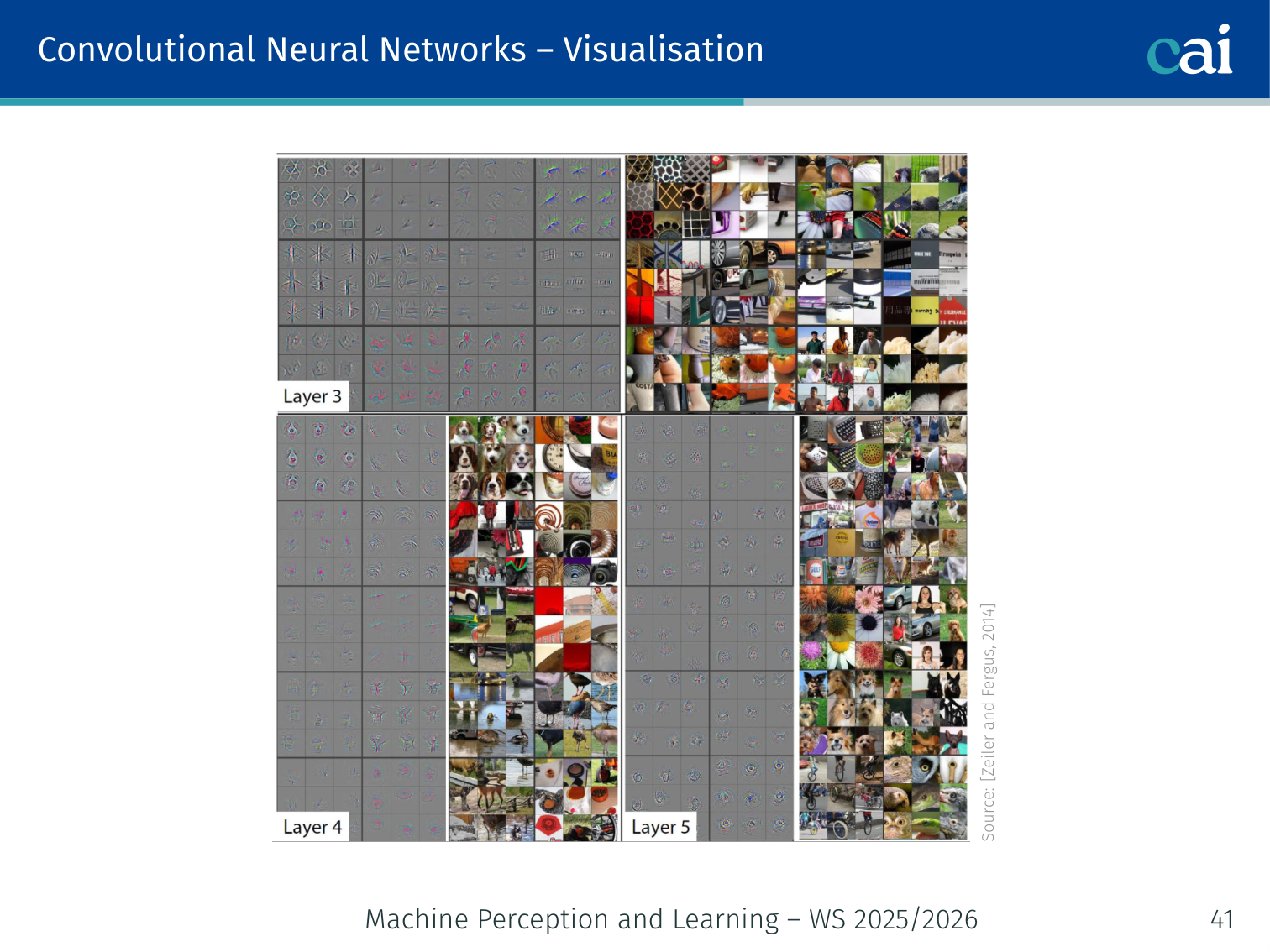
Later layers start recognizing complex parts and eventually whole objects.

[Zeiler and Fergus, 2014] — visualising what each filter responds to shows that:

Early layers learn edges, colors, and textures
Later layers learn more complex object parts and eventually whole objects

Brain/Neuron View

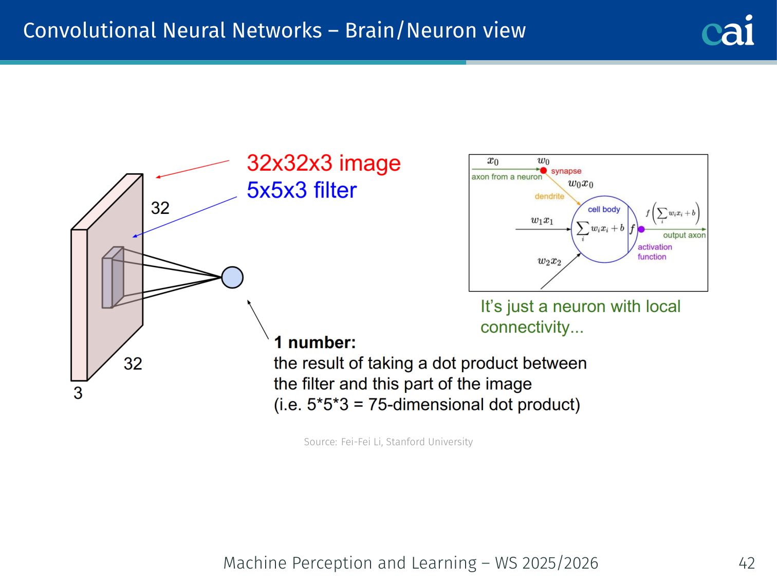
CNN feature maps are actually very similar to how V1 cells work in our brains.

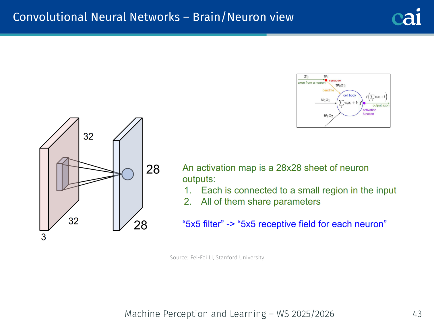
Both real and artificial neurons only "see" a small, local patch of the world.

Each unit in a feature map is connected only to a local patch of the input (its receptive field). Units sharing a filter form a layer analogous to a sheet of simple cells in V1.

Pooling Layer

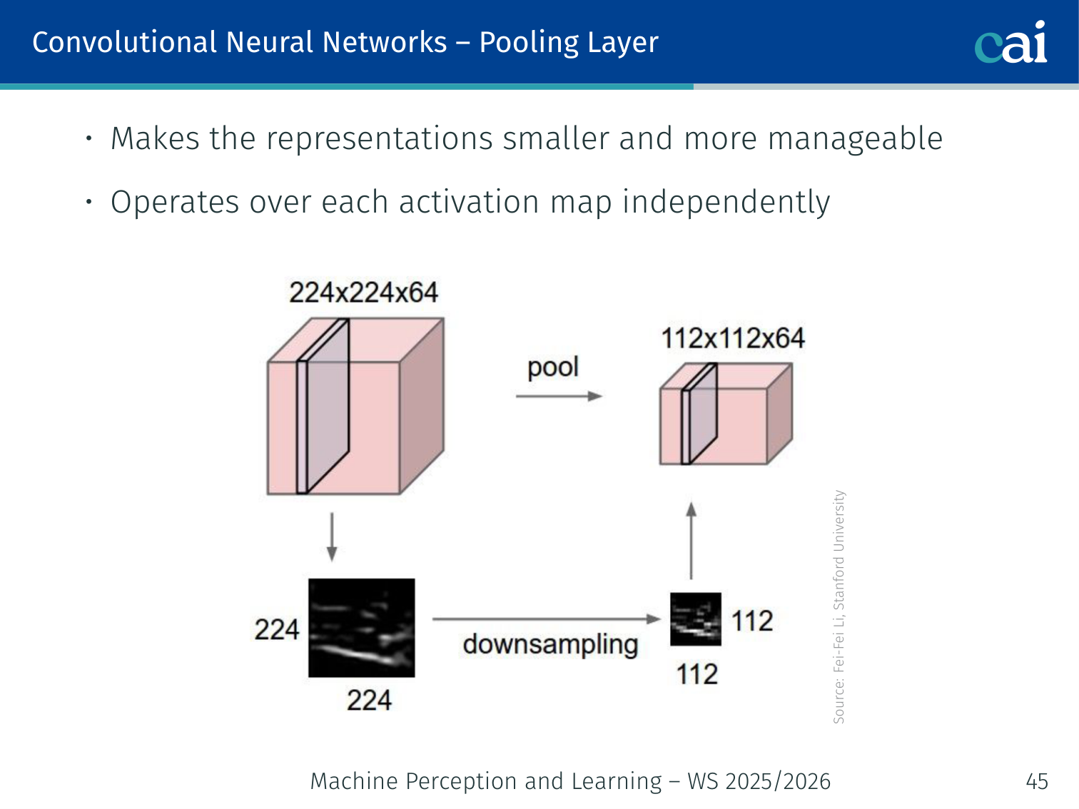
Pooling layers shrink the data to make it more manageable and less sensitive to shifts.

Makes representations smaller and more manageable
Operates over each activation map independently

Max pooling: takes the maximum value in each pooling window — the most common form.

Example — max pooling: if a 2×2 activation patch is $[0.1 0.2 0.7 0.6]$ , max pooling outputs 0.7. If the strongest response shifts slightly within that same window, the pooled output stays almost unchanged, which is why pooling gives small translation invariance.

Revolution of Depth

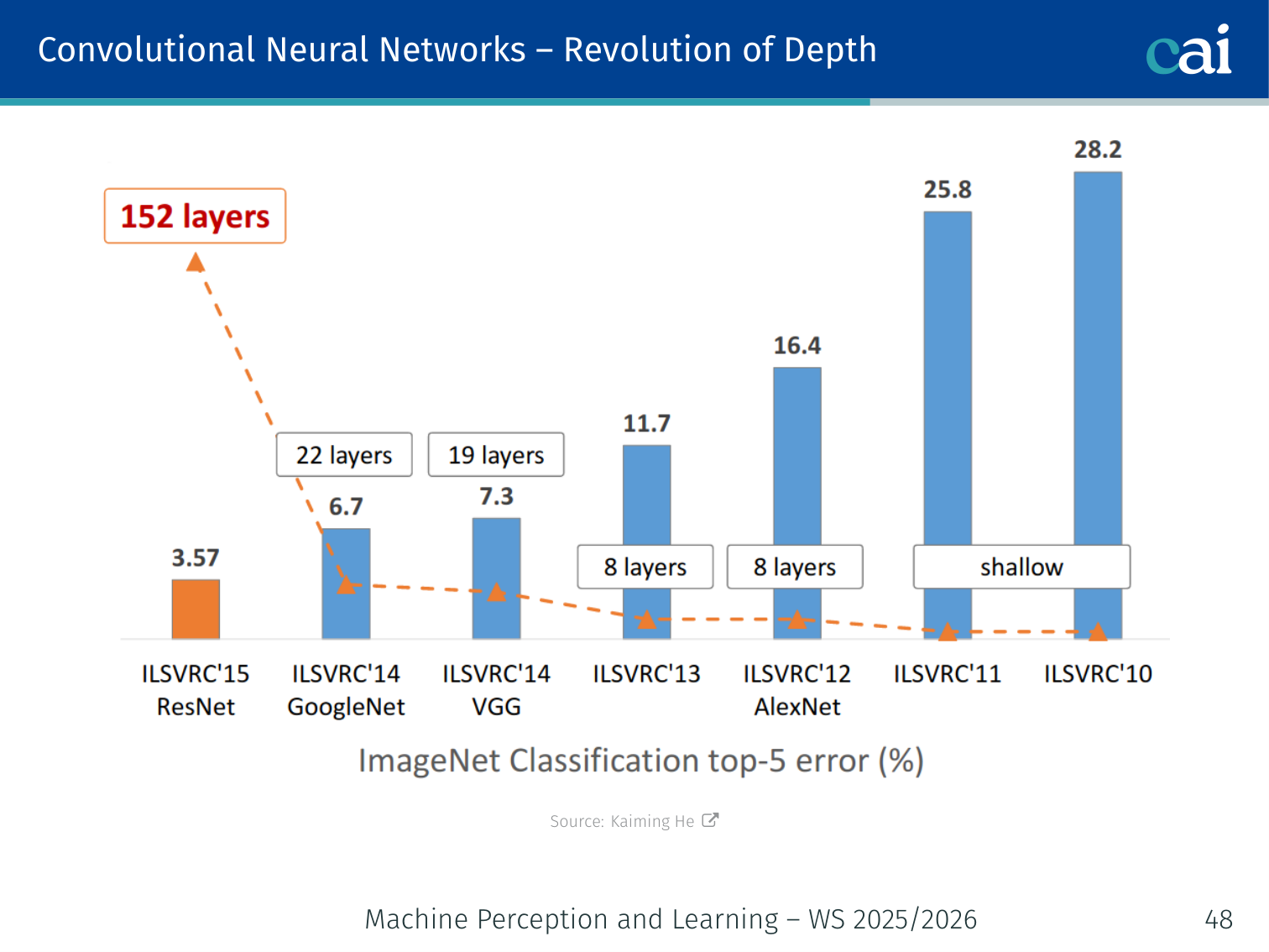
The "revolution of depth"—how networks have gotten way deeper over time.

How adding more layers has consistently slashed error rates on ImageNet.

Increasing network depth has been the primary driver of performance improvements in image recognition.

Case Study: VGG

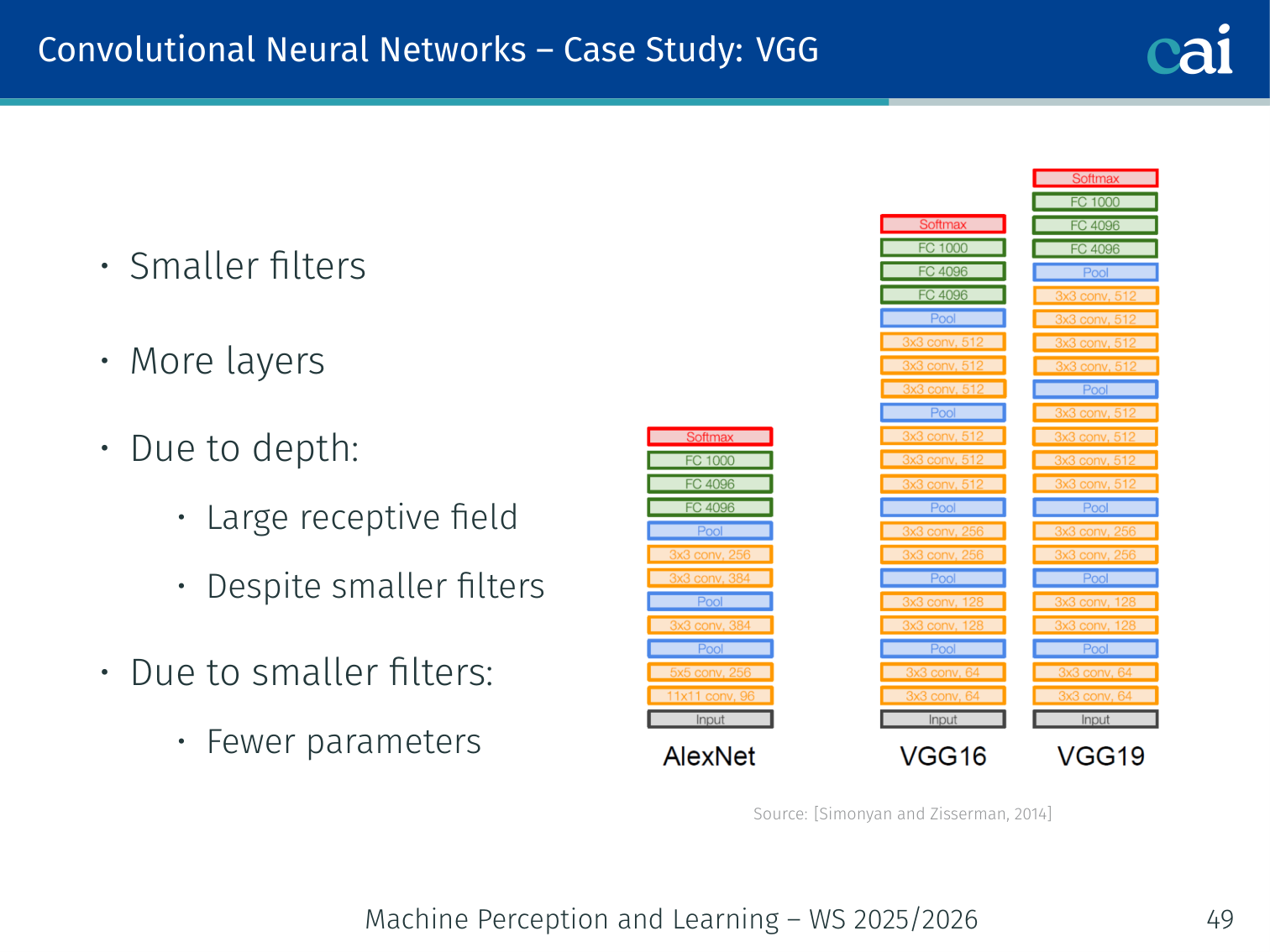
VGG showed that stacking lots of simple 3x3 filters is a winning strategy.

[Simonyan and Zisserman, 2014]

Smaller filters (only 3×3), more layers
Due to depth: large receptive field despite smaller filters
Due to smaller filters: fewer parameters

Case Study: GoogLeNet

The Inception module: a clever way to do multiple convolutions at once.

Comparing GoogLeNet's efficiency and depth against older models.

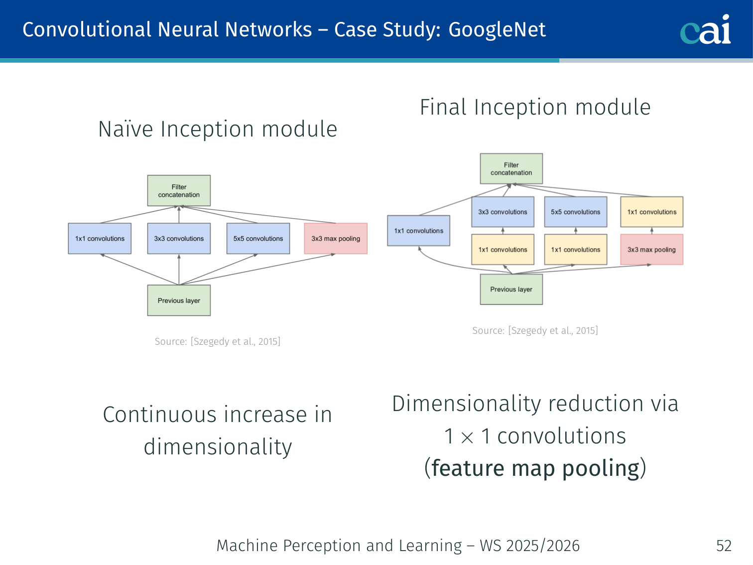
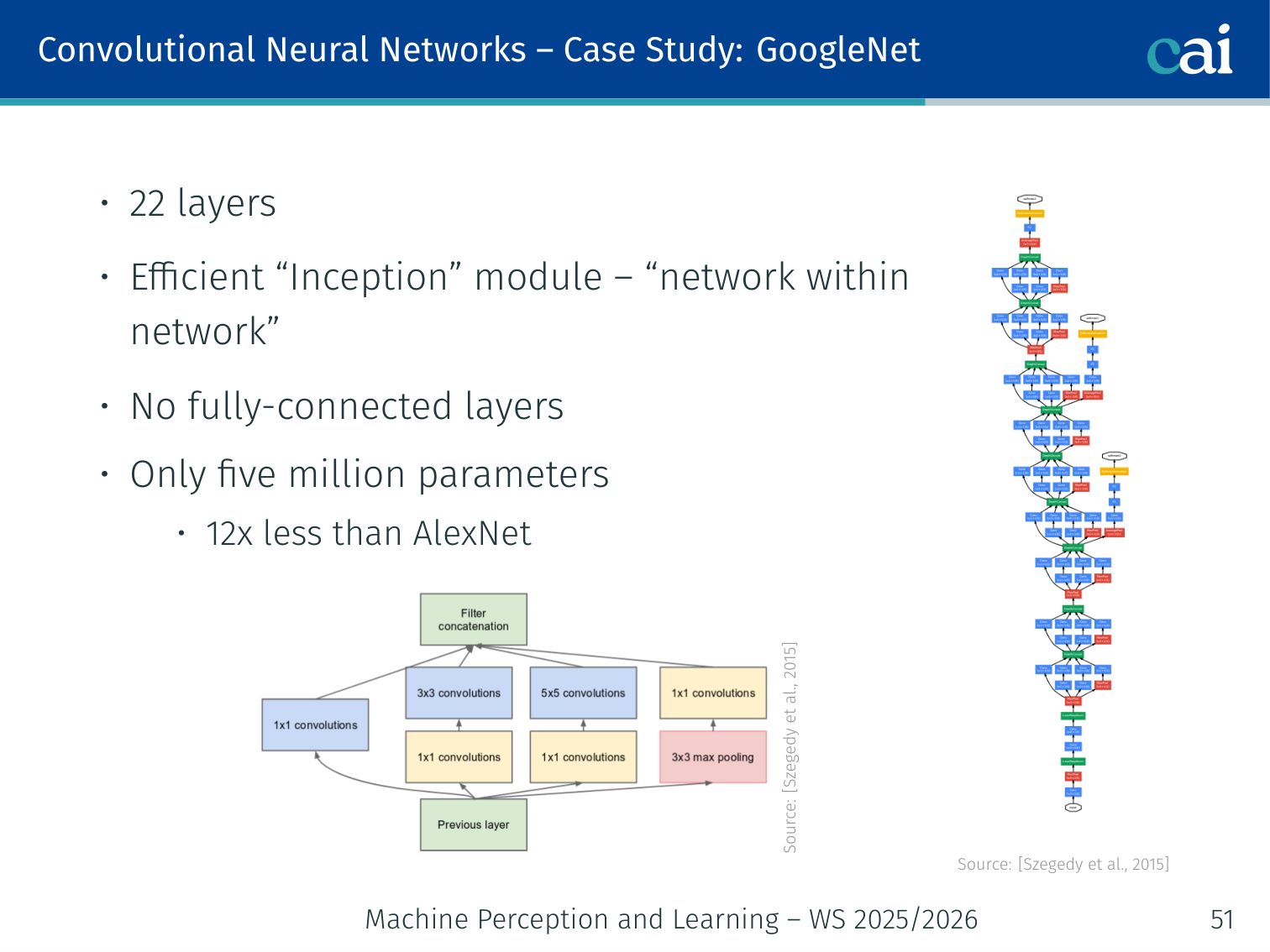
[Szegedy et al., 2015]

22 layers; efficient “Inception” module — “network within a network”
No fully-connected layers; only 5 million parameters (12× less than AlexNet)
Naïve Inception module: applies 1×1, 3×3, and 5×5 convolutions in parallel → continuous increase in dimensionality
Final Inception module: adds 1×1 convolutions for dimensionality reduction (feature map pooling) before expensive convolutions

Gradient Flow Problem

The "vanishing gradient" problem that makes training very deep networks so hard.

Ensuring sufficient gradient flow through very deep networks was a key challenge:

VGG: first trained an 11-layer model to convergence, then added random layers in the middle
GoogLeNet: used auxiliary classifiers to inject extra gradient into the lower layers

Shortly afterwards, batch normalisation was invented, removing the need for such hacks.

Case Study: ResNet

ResNet's skip connections let the gradient flow through dozens or even hundreds of layers.

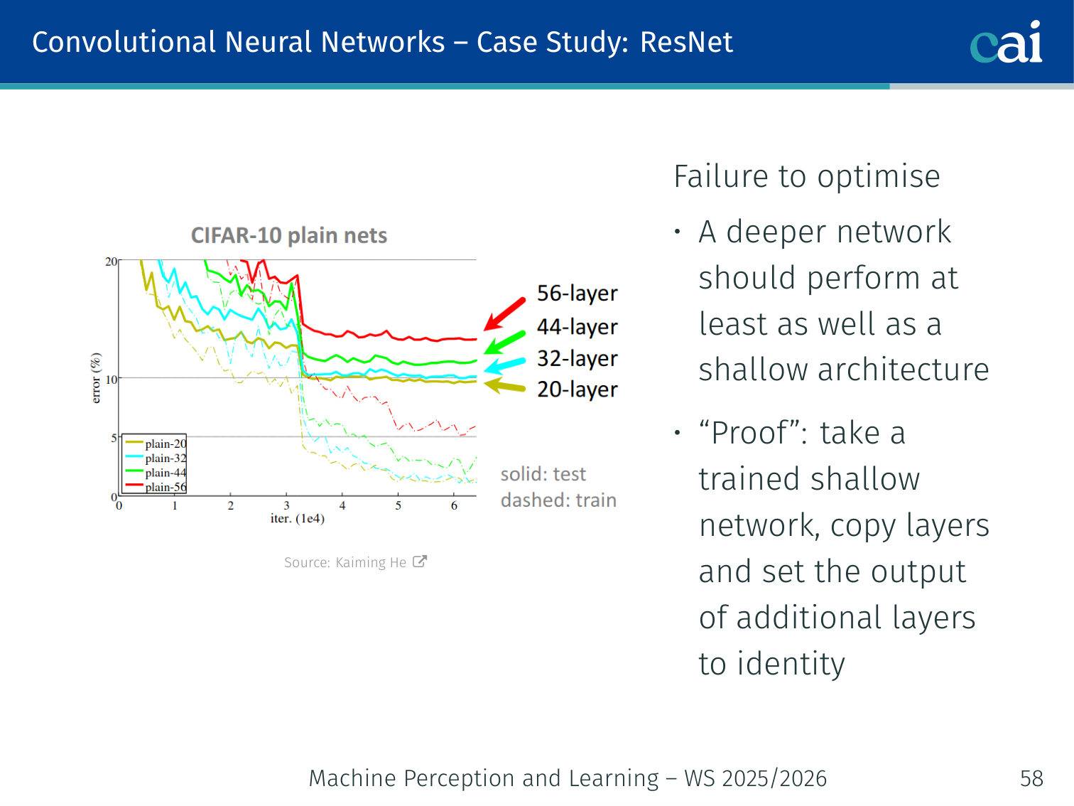
[He et al., 2016]

A deeper network should perform at least as well as a shallower one — in theory, you could take a trained shallow network, copy its layers, and set the extra layers to the identity. But in practice, optimisers fail to find this.

Residual connections fix this:

$y = F (x) + x$

$F (x)$ is a residual mapping w.r.t. identity.

Example — learning a correction instead of a full mapping: if earlier layers already detect a useful edge map, a later residual block only needs to learn a small change like “emphasize curved edges” or “suppress background texture”. That is much easier than relearning the entire representation from scratch.

If identity is optimal, it is easy to push $F (x)$ weights to 0
If the optimal mapping is close to identity, it is easier to learn small fluctuations
Residual connections improve gradient flow: at add-gates in the backward pass, the upstream gradient flows directly through the skip connection

Results:

Deep ResNets can be trained without difficulty
Deeper ResNets achieve lower training and lower test error
Trained in 2–3 weeks on an 8-GPU machine; faster than VGG at runtime despite being 8× deeper

Case Study: DenseNet / FractalNet

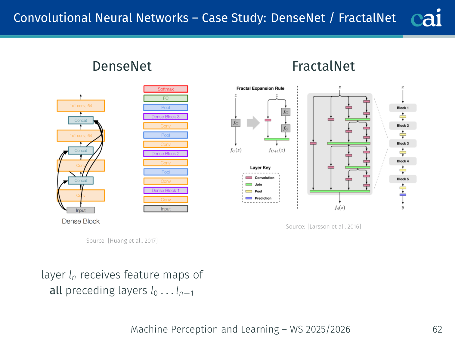
DenseNet and FractalNet take feature reuse to the extreme.

[Huang et al., 2017; Larsson et al., 2016]

DenseNet: layer $l_{n}$ receives feature maps from all preceding layers $l_{0} \dots l_{n - 1}$ — maximises feature reuse and gradient flow.

FractalNet: a fractal-structured network that achieves depth without residual connections.

Further Architectures

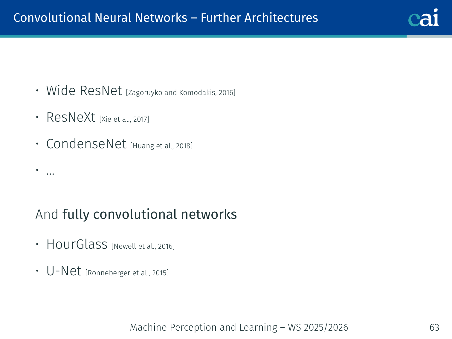
A quick look at some other popular architectures like Wide ResNet and ResNeXt.

Wide ResNet [Zagoruyko and Komodakis, 2016]
ResNeXt [Xie et al., 2017]
CondenseNet [Huang et al., 2018]

Fully convolutional networks for dense prediction:

HourGlass [Newell et al., 2016]
U-Net [Ronneberger et al., 2015]

PyTorch Implementation: LeNet-5

LeNet-5 is a classic CNN architecture for digit recognition. Below is its implementation in PyTorch.

import torch
import torch.nn as nn
import torch.nn.functional as F
 
# 1. Define the LeNet-5 Architecture
# Inheriting from nn.Module allows PyTorch to track parameters
class LeNet5(nn.Module):
    def __init__(self):
        super().__init__()
 
        # --- FEATURE EXTRACTION (Convolutional Layers) ---
 
        # Layer 1: Conv2d(in_channels=1, out_channels=6, kernel_size=5)
        # Input: 28x28 grayscale image (1 channel)
        # Output: 6 feature maps, each 24x24 (due to no padding)
        self.conv1 = nn.Conv2d(1, 6, kernel_size=5)
 
        # Layer 2: Conv2d(in_channels=6, out_channels=16, kernel_size=5)
        # Input: 6 feature maps from previous layer (after pooling)
        # Output: 16 feature maps
        self.conv2 = nn.Conv2d(6, 16, kernel_size=5)
 
        # --- CLASSIFICATION (Fully Connected Layers) ---
 
        # After two 2x2 pooling layers, a 28x28 image becomes 4x4
        # Flattened input features = channels (16) * height (4) * width (4) = 256
        self.fc1 = nn.Linear(16 * 4 * 4, 120)
        self.fc2 = nn.Linear(120, 84)
        # Output layer: 10 neurons for the 10 digits (0-9)
        self.fc3 = nn.Linear(84, 10)
 
    def forward(self, x):
        # Apply first convolution, then ReLU activation, then Max Pooling (2x2)
        # Resulting size: (28-5+1)/2 = 12x12
        x = F.max_pool2d(F.relu(self.conv1(x)), 2)
 
        # Apply second convolution, ReLU, and Max Pooling
        # Resulting size: (12-5+1)/2 = 4x4
        x = F.max_pool2d(F.relu(self.conv2(x)), 2)
 
        # Flatten: transform 4D tensor (Batch, 16, 4, 4) -> 2D (Batch, 256)
        x = x.view(-1, 16 * 4 * 4)
 
        # Standard fully connected feed-forward passes
        x = F.relu(self.fc1(x))
        x = F.relu(self.fc2(x))
 
        # Final output (logits) - CrossEntropyLoss will apply Softmax internally
        return self.fc3(x)

Key PyTorch CNN Functions:

nn.Conv2d: Learns spatial filters. It preserves the local relationship between pixels.
F.max_pool2d: Selects the maximum value in a small window, reducing spatial size and providing robustness to small translations.
x.view(-1, ...): Used to “flatten” the 2D feature maps into a 1D vector before passing them to traditional linear layers.

Applied Exam Focus

Dimension Formula: Output size $= \frac{W - K + 2 P}{S} + 1$ . Remember this to calculate feature map shrinkage.
Pooling: Max Pooling provides local translation invariance and reduces the number of parameters (lowering overfitting risk).
Receptive Field: Each layer increases the ‘view’ of the original image. Deeper layers capture more global context but lose spatial precision.

Previous: L01 — Intro | Back to MPL Index | Next: (y-03) Vision CNNs | (y) Return to Notes | (y) Return to Home

Yusuf's Thoughts

Explorer