L03 — CNNs in Computer Vision

Previous: L02 — CNNs | Back to MPL Index | Next: (y-04) RNNs

Mental Model First

• This lecture extends plain classification into structured vision tasks where we need to know not just what is present, but also where it is.
• Object detection adds bounding boxes; semantic segmentation adds a class label to every pixel.
• Most modern vision systems are really about designing a good tradeoff between speed, precision, and output granularity.
• If one question guides this lecture, let it be: how do CNN features get turned into spatial predictions instead of just one final class label?

Case Study: EfficientNet

EfficientNet asked a simple scaling question: if we are allowed more compute, should we make a CNN deeper, wider, or feed it higher-resolution images? The key result was that these three dimensions should be scaled together, not independently (Tan and Le, 2019).

Compound Scaling

EfficientNet uses a single scaling coefficient $\varphi$ and scales depth, width, and resolution jointly:

$$\text{depth}={\alpha }^{\varphi },\text{width}={\beta }^{\varphi },\text{resolution}={\gamma }^{\varphi }$$

subject to the constraint

$$\alpha {\beta }^2{\gamma }^2\approx 2$$

so that each increment of $\varphi$ roughly doubles the compute budget in a balanced way.

Base Architecture from NAS

The base network, EfficientNet-B0, was found with Neural Architecture Search (NAS). Once B0 is fixed, larger variants B1-B7 are produced by compound scaling rather than redesigning the architecture by hand.

EfficientNet B0-B7

Model	Input resolution	Params	ImageNet top-1
B0	224	5.3M	77.1%
B1	240	7.8M	79.1%
B2	260	9.2M	80.1%
B3	300	12M	81.6%
B4	380	19M	82.9%
B5	456	30M	83.6%
B6	528	43M	84.0%
B7	600	66M	84.3%

This shows the intended tradeoff clearly:

• B0/B1: smaller and faster
• B4/B5: strong middle ground
• B6/B7: highest accuracy, but much more expensive

Example: Instead of only stacking more layers like a deeper ResNet, EfficientNet also increases channel width and image resolution, so the extra compute is spent more evenly across the model.

Why It Mattered

At the time, EfficientNet achieved better accuracy per FLOP than many ResNet-family models. The broader lesson was that balanced scaling is more efficient than blindly scaling depth alone.

---

Object Detection

What is it?

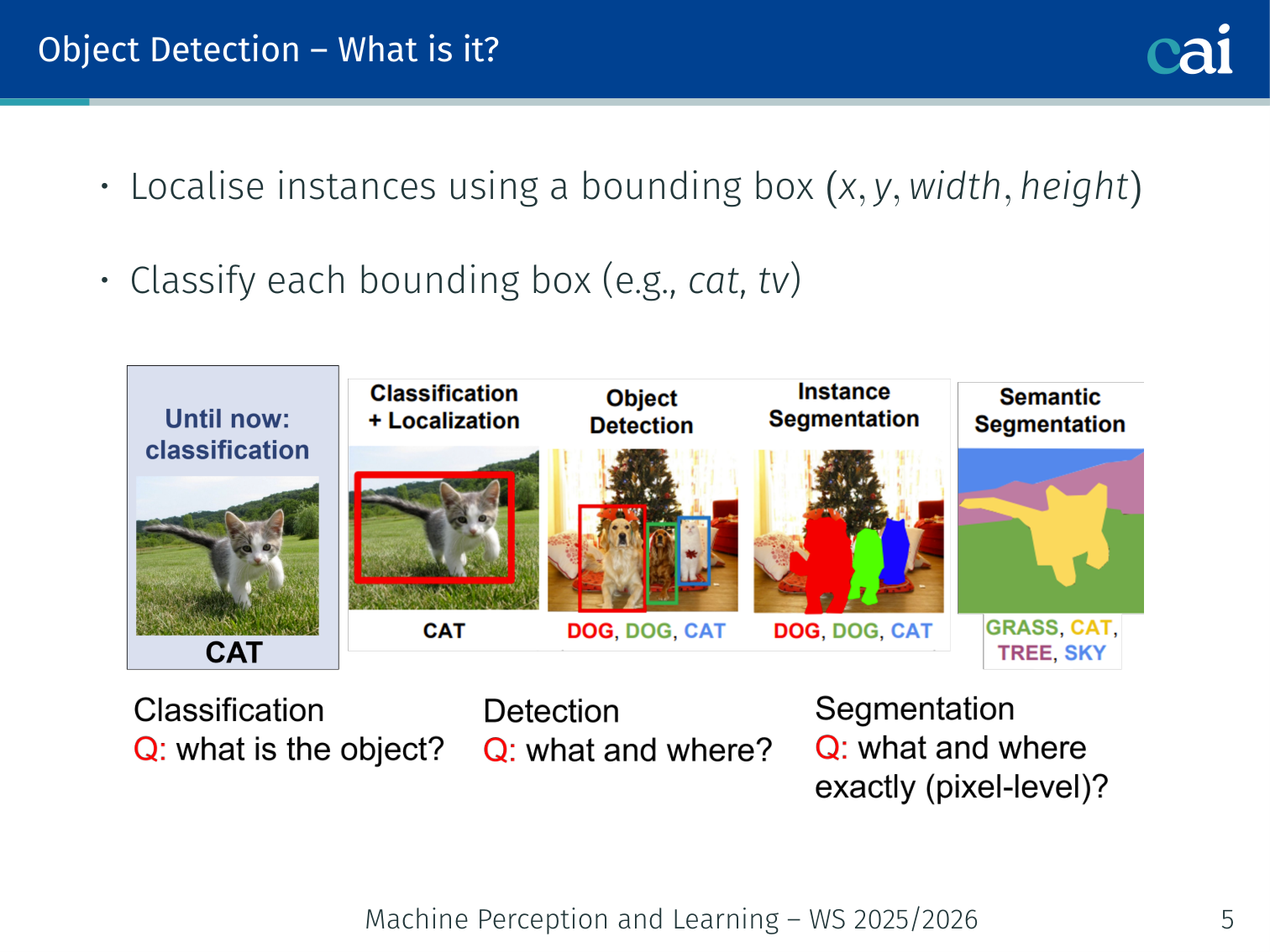
Object detection is about both identifying what's in the image and where it is.

• Localise instances using a bounding box $(x,y,\text{width},\text{height})$
• Classify each bounding box (e.g., cat, tv)

Why do we need it?

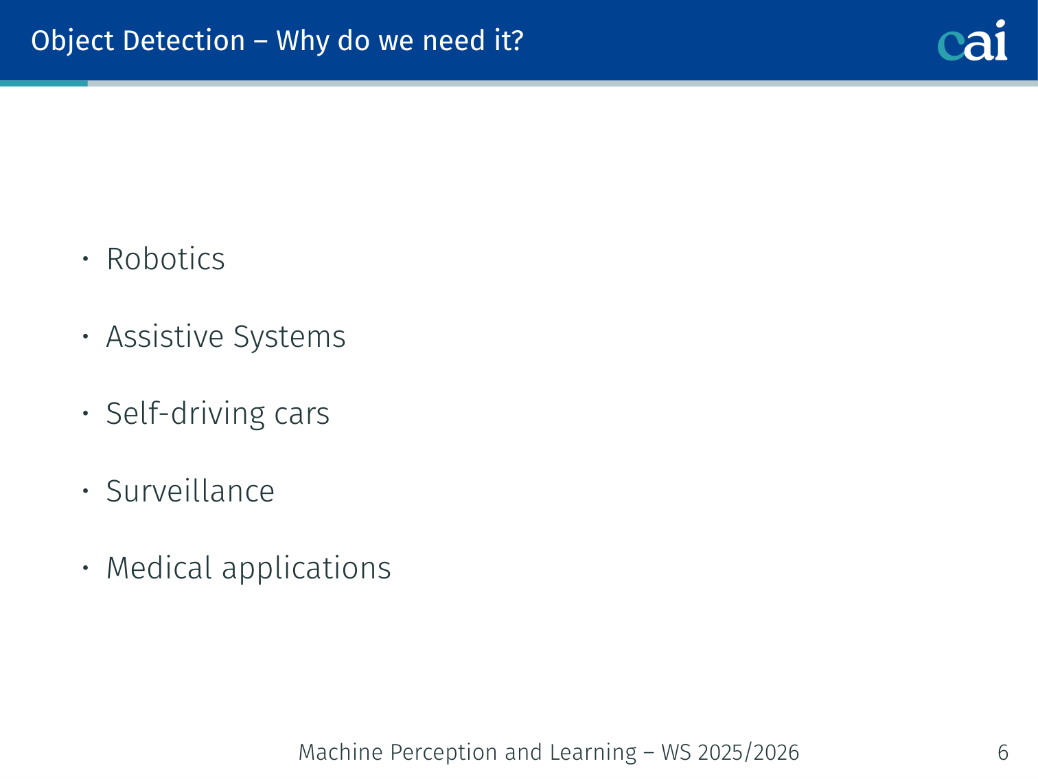
We use object detection for everything from self-driving cars to medical imaging.

Robotics, assistive systems, self-driving cars, surveillance, medical applications.

---

Classification vs. Regression — Recap

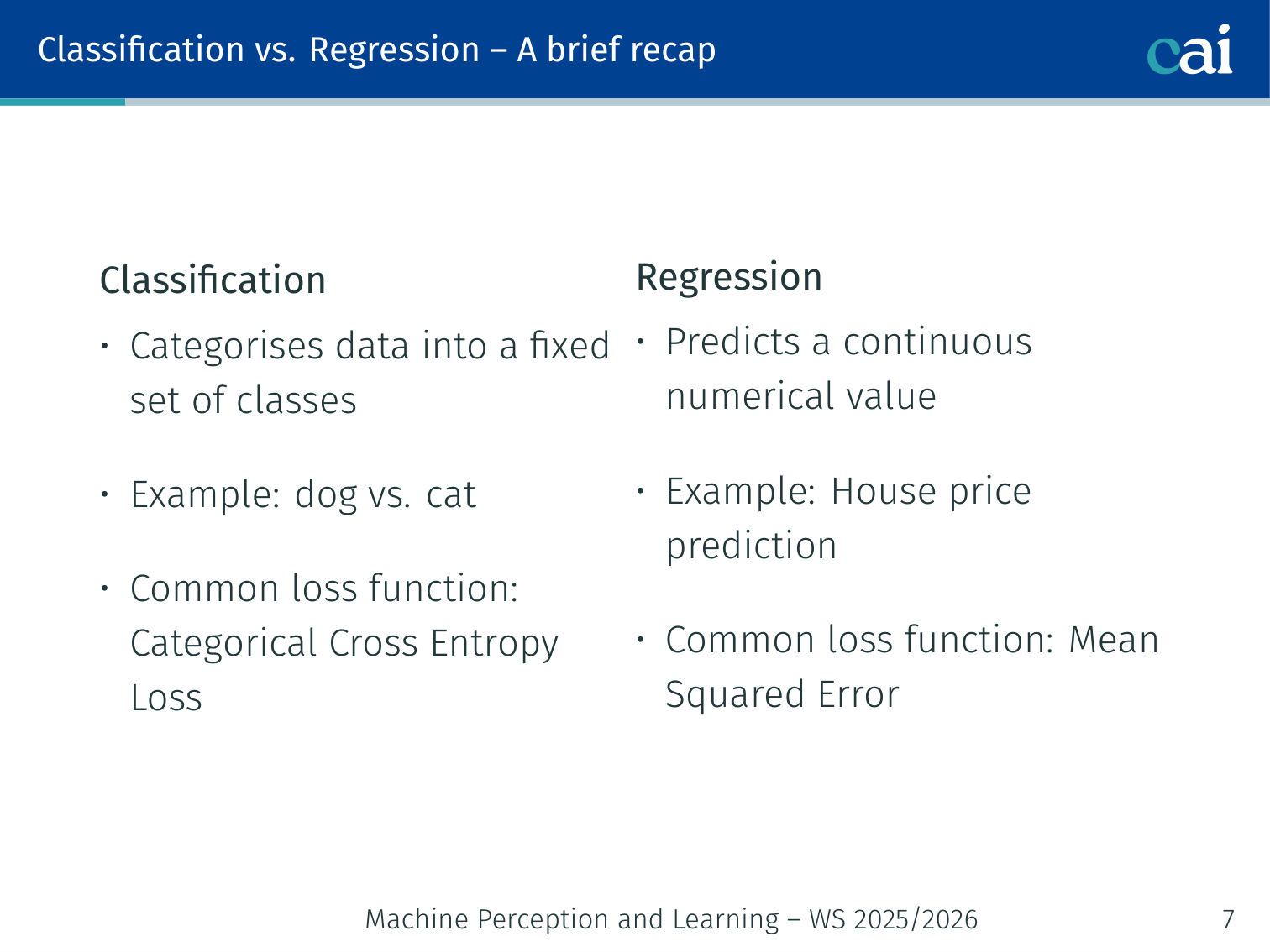
A quick refresher on the difference between classification and regression.

Classification: categorises data into a fixed set of classes (e.g., dog vs. cat). Common loss: categorical cross-entropy.

Regression: predicts a continuous numerical value (e.g., house price, bounding-box coordinates). Common loss: mean squared error.

Example — regression output: a model taking a 224×224 image and outputting [0.3, 0.5, 0.2, 0.4] for a single box’s $(x,y,w,h)$.
Problem: the number of objects varies per image, so the output size is variable — a fixed regression layer can’t handle this directly.

---

Detection as a Regression Problem

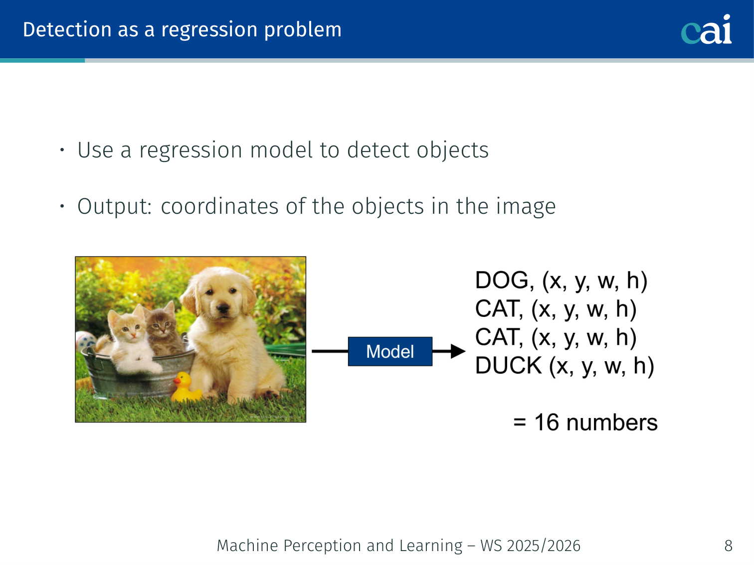
Trying to treat object detection as a simple regression problem to find coordinates.

Use a regression model to detect objects — output: coordinates of the objects in the image.

Problem: need variable-sized outputs (different images contain different numbers of objects).

---

Detection as a Classification Problem

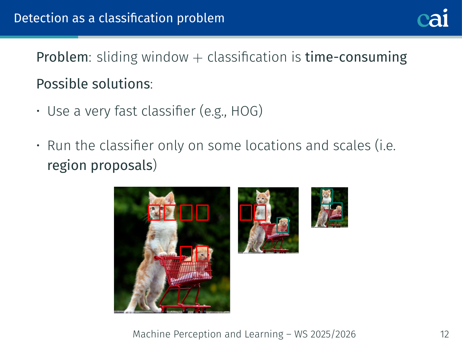
Another way: treating detection as a classification task with a sliding window.

Use a sliding window:

• Move a small window across the image at every position and scale
• Run a classifier on each patch to assign an object class

Problem: applying the classifier at all positions and scales is extremely time-consuming.

Possible solutions:

• Use a very fast classifier (e.g., HOG)
• Run the classifier only on some locations and scales → region proposals

---

Region Proposal Methods

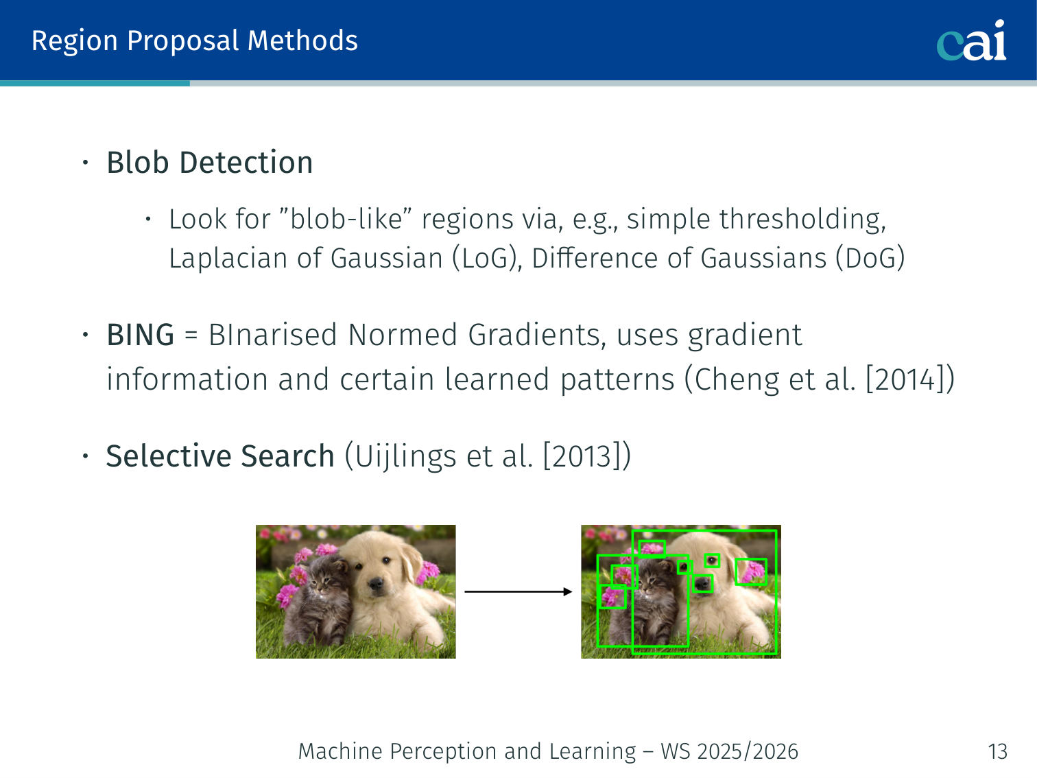
A look at methods like Selective Search that suggest where objects might be.

• Blob Detection: look for “blob-like” regions via, e.g., simple thresholding, Laplacian of Gaussian (LoG), Difference of Gaussians (DoG)
• BING (BInarised Normed Gradients) [Cheng et al., 2014]: uses gradient information and learned patterns; runs at 300 fps
• Selective Search [Uijlings et al., 2013]: bottom-up hierarchical grouping
  • Split image based on colour into initial regions
  • Iteratively merge neighbouring regions based on similarity
  • Produces a hierarchy of region proposals at multiple scales

Example — Selective Search: an image of a dog on a grass field might first be segmented by colour into ~200 regions (brown patch = dog body, green = grass). Nearby similar regions merge iteratively until we have a small set of candidate boxes, one of which tightly covers the dog. This is much faster than dense sliding window search.

Key idea: fast + dense generic detection with selective search, then slow + sparse classification on just the proposals.

---

R-CNN [Girshick et al., 2014]

R-CNN: the first big model to use region proposals with a CNN.

Region-based CNN — only feeds proposed regions to a classifier.

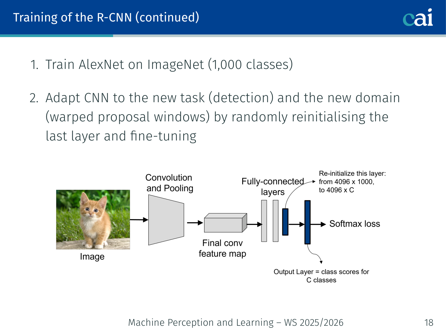
Training pipeline:

1. Pre-train AlexNet on ImageNet (1,000 classes)
2. Adapt (fine-tune) the CNN to the detection task and the domain of warped proposal windows — reinitialise the last layer and fine-tune
3. Train SVMs: binary SVM per object class using pool5 features of the fine-tuned AlexNet as inputs
4. Train a bounding-box regressor: input = pool5 features of the proposed region; output = refined $(x,y,\text{width},\text{height})$

Example flow: ~2,000 region proposals per image, each warped to 227×227 and fed through AlexNet → pool5 features → 20 SVMs (one per VOC class) + box regressor.

The lecture’s result slide makes the core contribution visible: once proposals are cropped and passed through a fine-tuned CNN, the detector can localise many Pascal VOC objects quite tightly across very different categories. The tradeoff is efficiency: every proposal still requires its own CNN forward pass, which makes test-time inference extremely slow.

---

Fast R-CNN [Girshick, 2015]

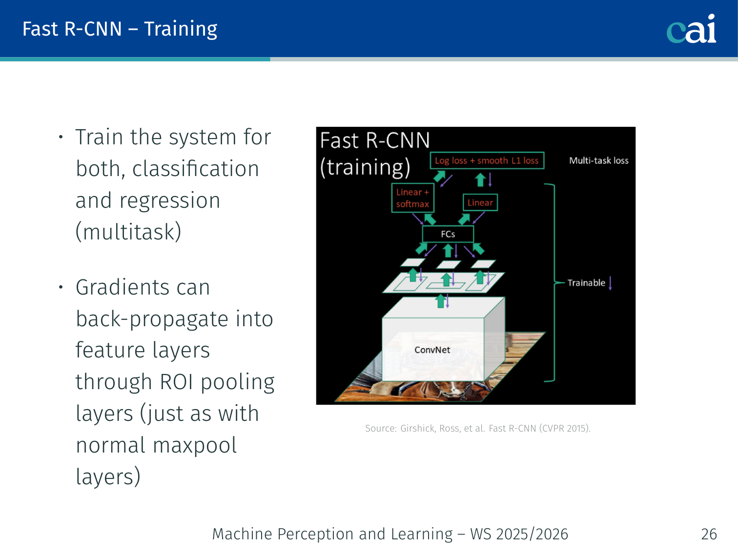
Fast R-CNN made things way faster by sharing feature maps across all proposals.

Key improvement: compute the CNN feature map once for the whole image, then extract per-proposal features from it.

RoI Pooling: project a region proposal onto the shared feature map → max-pool to a fixed-size output (e.g., 7×7), regardless of the proposal’s input size.

• Unified network: single forward pass jointly optimises classification and bounding-box regression (multitask loss)
• Gradients back-propagate through RoI Pooling into the feature layers (just like normal MaxPool)
• Slight accuracy improvement from end-to-end training

Downside: the majority of runtime is still spent on region proposals (Selective Search is outside the network).

Example: for a 600×1000 image, one CNN forward pass produces a feature map; 2,000 RoI Pooling operations each take ~6ms, whereas Selective Search takes ~2 seconds.

---

Faster R-CNN [Ren et al., 2015]

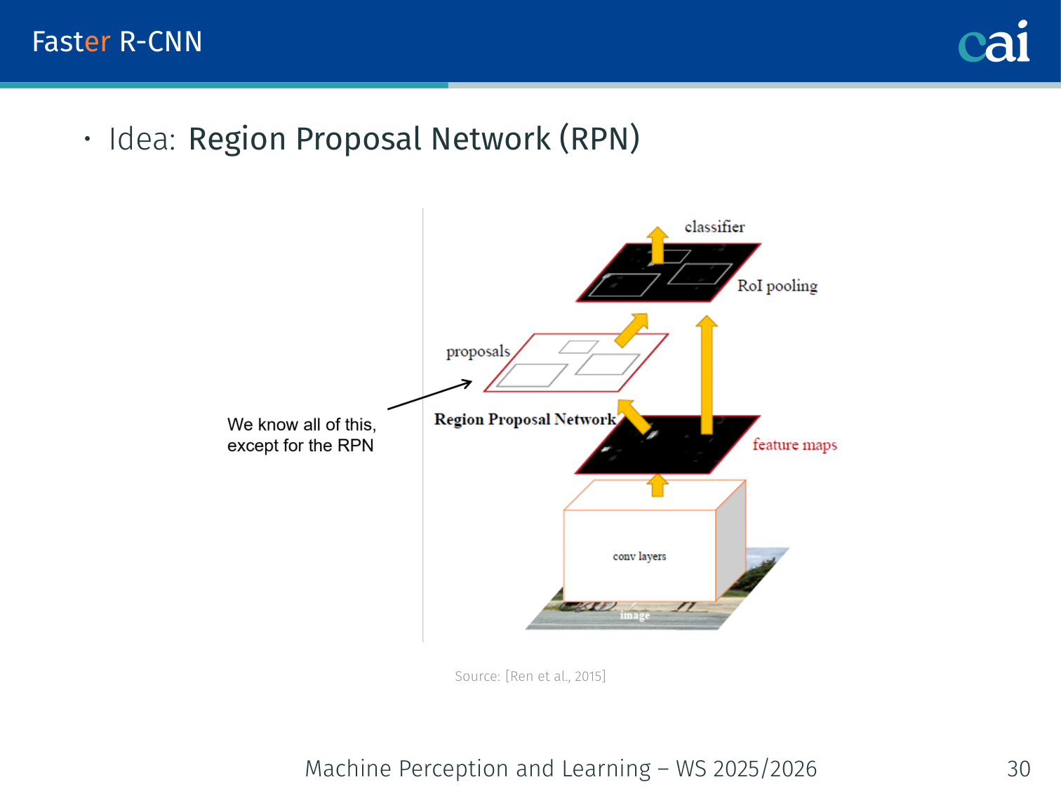
Faster R-CNN brought region proposals directly into the network with the RPN.

Eliminates the external region proposal step by adding a Region Proposal Network (RPN) that runs on the same feature map as the detector.

Region Proposal Network (RPN)

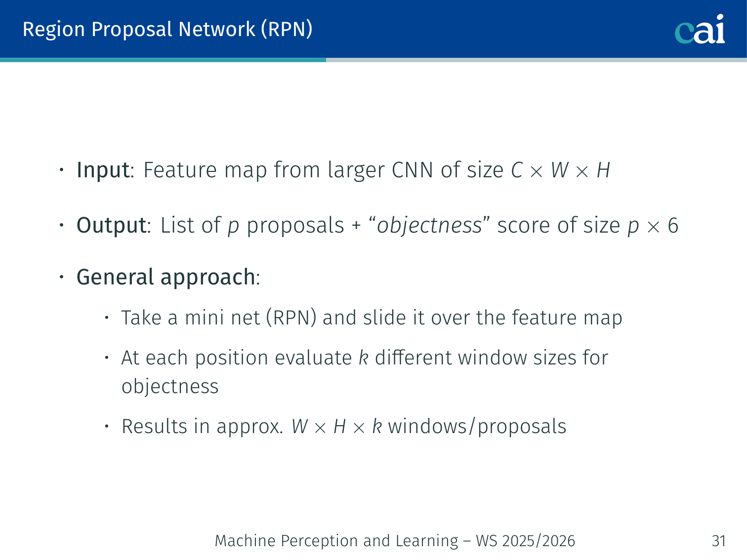
A closer look at the RPN, the part of the network that "guesses" where objects are.

• Input: feature map from the backbone CNN of size $C\times W\times H$
• Output: list of $p$ proposals + “objectness” score; output size $p\times 6$
• Approach: slide a small (mini) net over the feature map; at each position evaluate $k$ different window sizes for objectness → $\approx W\times H\times k$ proposals

💡 Intuition: Anchors as “Starting Guesses”

Imagine you are looking for objects in a foggy field. Instead of searching every square inch, you place a few differently sized hula-hoops (Anchors) at fixed spots on the ground.

• The Question: “Does anything in this hula-hoop look like an object?”
• The Adjustment: If the answer is “yes”, you don’t just take the hula-hoop as it is. You “nudge” it (Bounding Box Regression) to fit the object perfectly.

This is much faster than trying to draw a new box from scratch at every single pixel.

---

Anchors:

• Initial reference boxes defined by aspect ratio and scale, centred at each sliding window position
• 3 scales × 3 aspect ratios = 9 anchors per position
• reg head: regression of anchor coordinates; cls head: object / no-object score

Example: for a 38×50 feature map (stride 16 from a 600×800 image) and 9 anchors, the RPN evaluates 38 × 50 × 9 = 17,100 candidate boxes per image.

Labelling Anchors:

• Positive anchor: highest IoU with a ground-truth box, OR IoU > 0.7
• Negative anchor: IoU < 0.3
• Other anchors do not contribute to training

IoU example: if a predicted box and a ground-truth box have an intersection area of 30 and a union of 100, IoU = 0.3 → classified as negative.

RPN Loss Function:

$L(p_i,t_i)=\frac{1}{N_{\text{cls}}}{\sum }_i{L}_{\text{cls}}(p_i,p_i^{\ast })+\lambda \frac{1}{N_{\text{reg}}}{\sum }_i{p}_i^{\ast }{L}_{\text{reg}}(t_i,t_i^{\ast })$

• $L_{\text{cls}}$: classification loss (object vs. background)
• $L_{\text{reg}}$: regression loss on box coordinates
• $N_{\text{cls}}$: batch size; $N_{\text{reg}}$: number of positive anchors (~2,040)
• $\lambda$: balancing weight

Result: ~10× speedup over Fast R-CNN with no loss in accuracy.

The R-CNN Family at a Glance

The lecture’s comparison slide highlights that the main progress from R-CNN → Fast R-CNN → Faster R-CNN is about eliminating repeated computation while preserving accuracy:

Model	Test time / image (with proposals)	Speedup	mAP (VOC 2007)
R-CNN	50 s	1×	66.0
Fast R-CNN	2 s	25×	66.9
Faster R-CNN	0.2 s	250×	66.9

So the big story is not that Faster R-CNN suddenly becomes much more accurate; it achieves roughly the same detection quality with drastically less wasted computation.

The COCO qualitative examples in the PDF also show that the Faster R-CNN pipeline scales beyond the cleaner Pascal VOC setting: it can detect many objects simultaneously in cluttered indoor and outdoor scenes, from kitchen items and trains to animals and street scenes.

---

Segmentation Extension: Mask R-CNN [He et al., 2017]

Mask R-CNN takes Faster R-CNN a step further by adding per-pixel masks.

Extends Faster R-CNN with an additional instance-segmentation head:

• The classification stage gains an extra branch for predicting a per-pixel binary mask
• Further improves object detection results alongside providing instance masks

---

Single-Stage Detectors

Single-stage detectors like SSD and YOLO are built for maximum speed.

Two-stage detectors are accurate but slow. Single-stage detectors skip the proposal step.

SSD — Single Shot MultiBox Detector [Liu et al., 2016]:

• Directly predicts class scores and box offsets (no RPN)
• Uses default (anchor) boxes for predictions
• Detects objects at multiple scales using feature maps from different layers
• Combines multi-scale predictions for improved accuracy over objects of varying sizes

YOLO — You Only Look Once [Redmon et al., 2016]:

• Divides the image into a grid (e.g., 13×13 for YOLOv3)
• Each grid cell predicts bounding boxes and class probabilities
• Processes images in a single forward pass → extremely fast
• Tends to miss small objects as it prioritises global context

Example — YOLO grid: divide a 416×416 image into a 13×13 grid. Each of the 169 cells outputs 5 candidate boxes with (x, y, w, h, confidence) + 80 class scores. The whole prediction runs in one forward pass at ~45 FPS.

---

Semantic Segmentation

What is it?

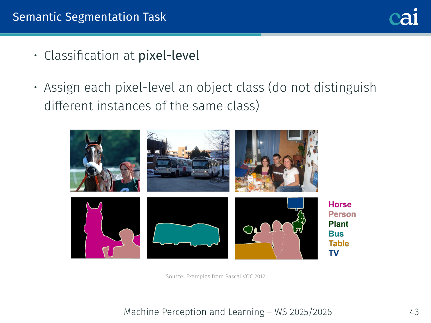
Semantic segmentation is all about giving every single pixel its own class label.

Classification at pixel-level: assign each pixel an object class label (e.g., road, sky, person). Does not distinguish different instances of the same class.

Example — Pascal VOC: an image with two people and a car would have every person-pixel labelled “person” and every car-pixel labelled “car” — both people share the same label colour.

It helps to separate the related tasks clearly:

Task	Output	Example
Image classification	One label for the whole image	”dog”
Object detection	One box + class per instance	two dogs → two boxes
Semantic segmentation	One class per pixel	both dogs share the same dog label region
Instance segmentation	One mask per object instance	each dog gets its own mask

---

Sliding Window Approach

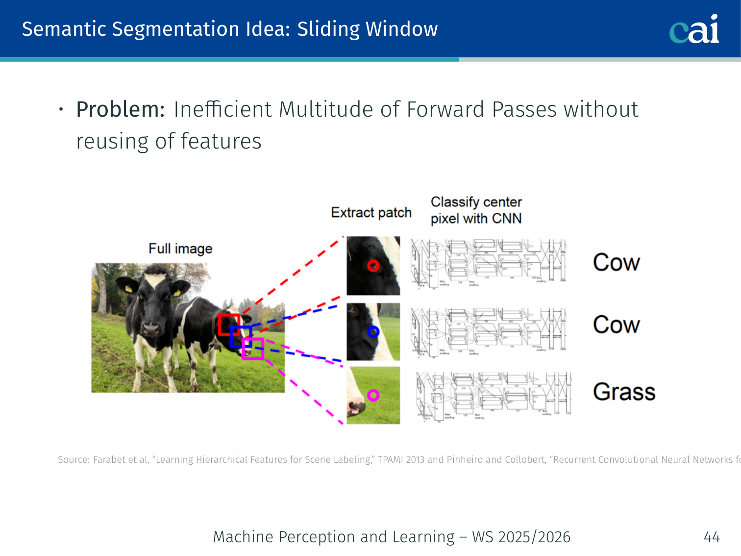
The old, slow way of doing segmentation with a sliding window.

Apply a patch classifier at every pixel location. Problem: inefficient — no sharing of computed features between overlapping patches; requires a multitude of forward passes.

---

Fully Convolutional Networks (FCN) [Long et al., 2015]

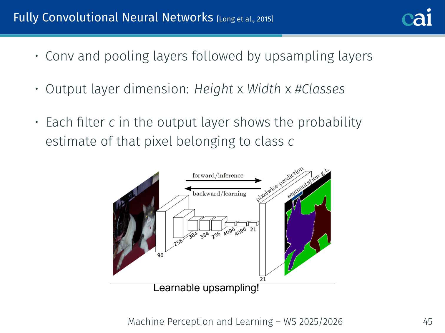
FCNs: networks that are convolutional all the way down for dense predictions.

• Convolution and pooling layers followed by upsampling layers
• Output layer dimension: $H\times W\times \#\text{Classes}$
• Each filter $c$ in the output layer gives the probability estimate of a pixel belonging to class $c$

Example: a 224×224 image with 21 VOC classes → output tensor of shape 224×224×21. argmax over the class dimension gives the final per-pixel class map.

---

In-Network Upsampling

Unpooling (Nearest-Neighbour)

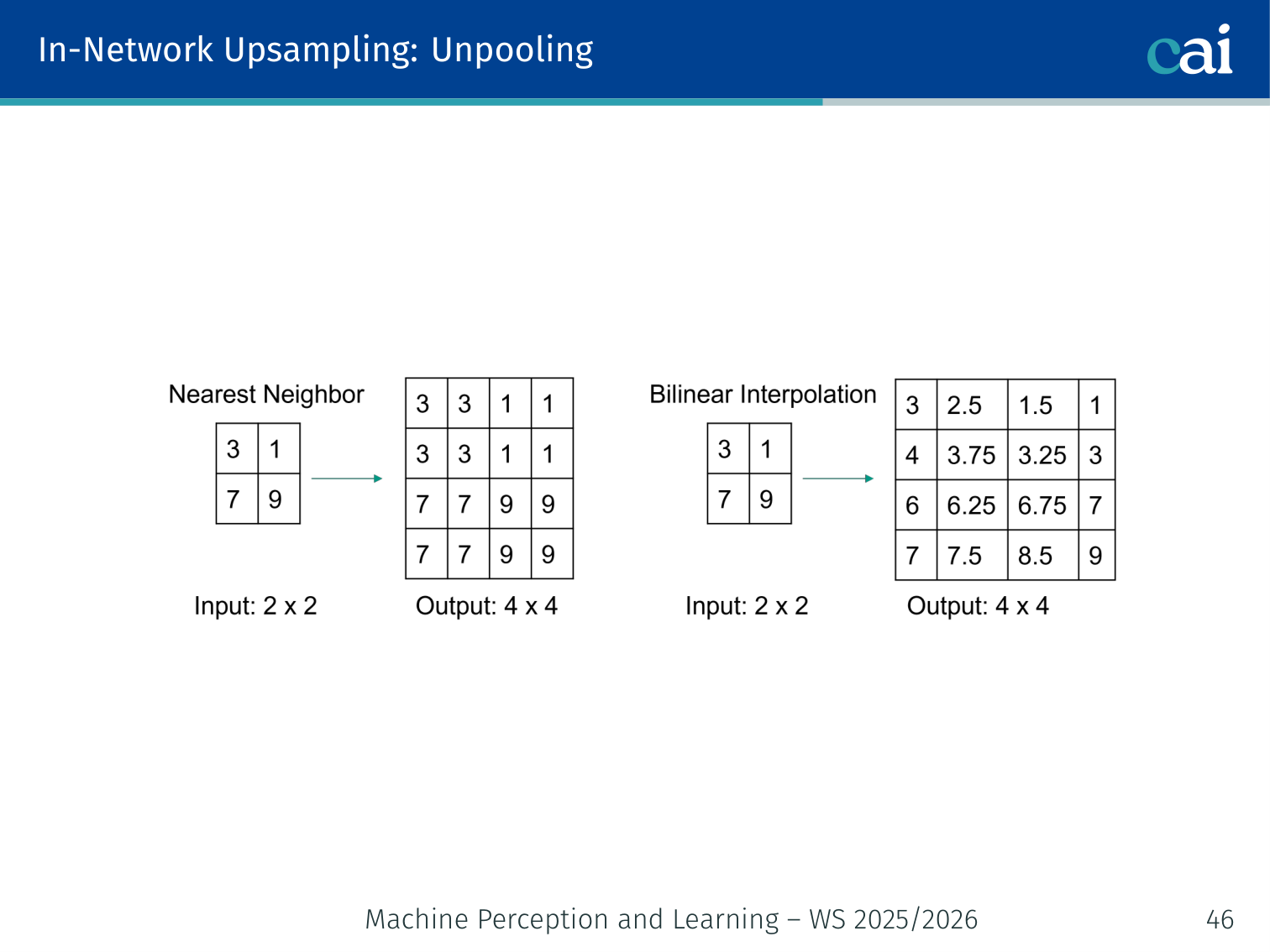
Nearest-neighbor unpooling: a simple, but blocky, way to resize an image.

Simply repeat (or tile) each value into the larger grid. Fast but blocky — no learned content.

Max Unpooling

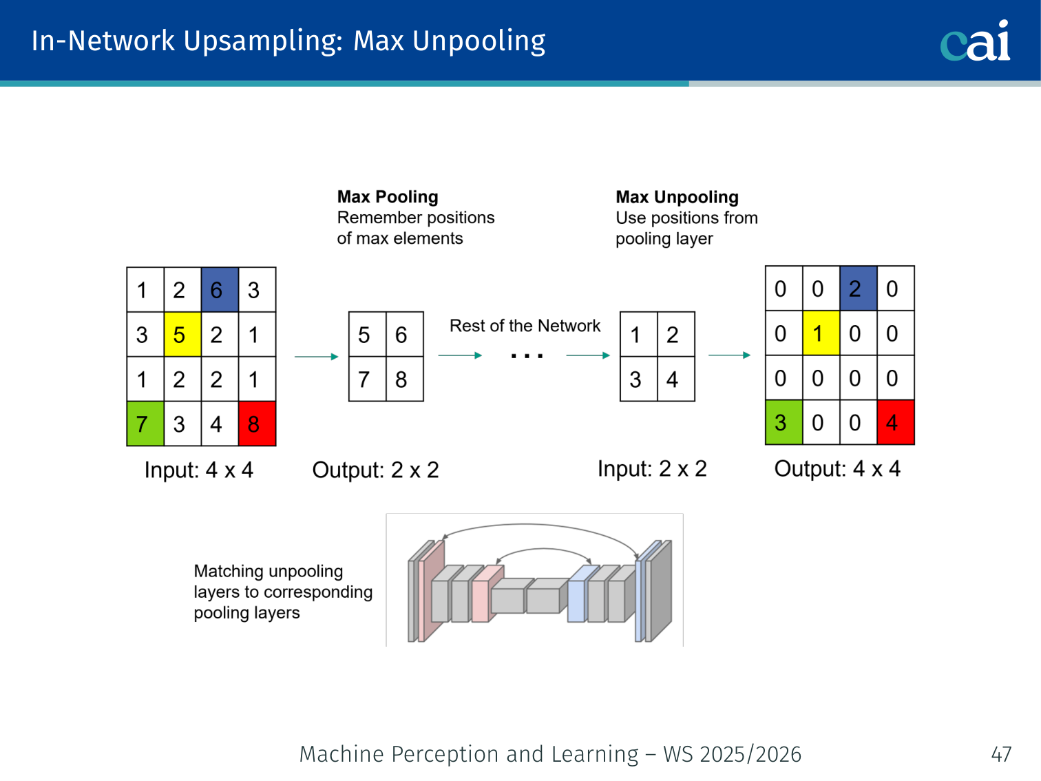
Max unpooling uses "switches" from the pooling layer to put pixels back where they belong.

During the forward max-pool, record the switch positions (which location held the max). During unpooling, place values back at those positions; all other locations are set to 0.

Example: 2×2 region [1, 3; 5, 2] → max pool selects 5, records position (1,0). During unpooling, 5 is placed at (1,0) and zeros fill the rest: [0, 0; 5, 0].

Transposed Convolution (Learnable Upsampling)

Transposed convolution lets the network learn the best way to upsample.

Using a learned kernel to intelligently fill in the gaps when upsampling.

• Insert zeros between input values (stride > 1 in the “input space”), then apply a learned convolution kernel
• The network learns how to upsample — can produce sharp, detailed outputs
• Also called “deconvolution” (though mathematically it is not a true deconvolution)

🧠 Deep Dive: Transposed Conv vs. Interpolation

When we want to make an image larger (upsample), we have two main choices:

1. Bilinear/Nearest Interpolation: This is a fixed mathematical formula. It’s fast, but it often results in “blurry” or “blocky” edges because it doesn’t “know” what it’s looking at.
2. Transposed Convolution: This is a learnable upsampling. The network learns a set of weights that decide how to fill in the gaps.
   • Pro: It can learn to reconstruct fine details (like the sharp edge of a road or a person’s silhouette).
   • Con: It can sometimes produce “checkerboard artifacts” if the kernel size and stride aren’t perfectly aligned.

---

Example — stride-2 transposed conv: a 2×2 input becomes 4×4 after inserting zeros between each input value, then a 3×3 learned filter sweeps over it.

---

Learning Deconvolution Network [Noh et al., 2015]

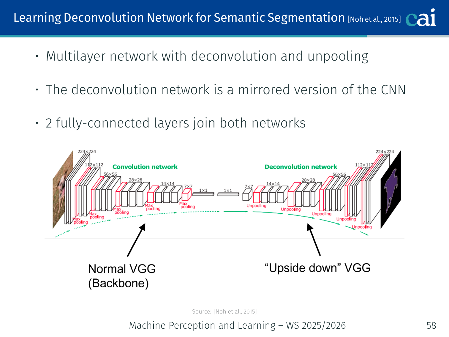
The Learning Deconvolution Network uses a nice, symmetric encoder-decoder structure.

• Multilayer network with alternating deconvolution and unpooling layers
• The deconvolution network is a mirrored version of the CNN (encoder → decoder)
• Two fully-connected layers join the encoder and decoder networks

---

FCN Skip Connections

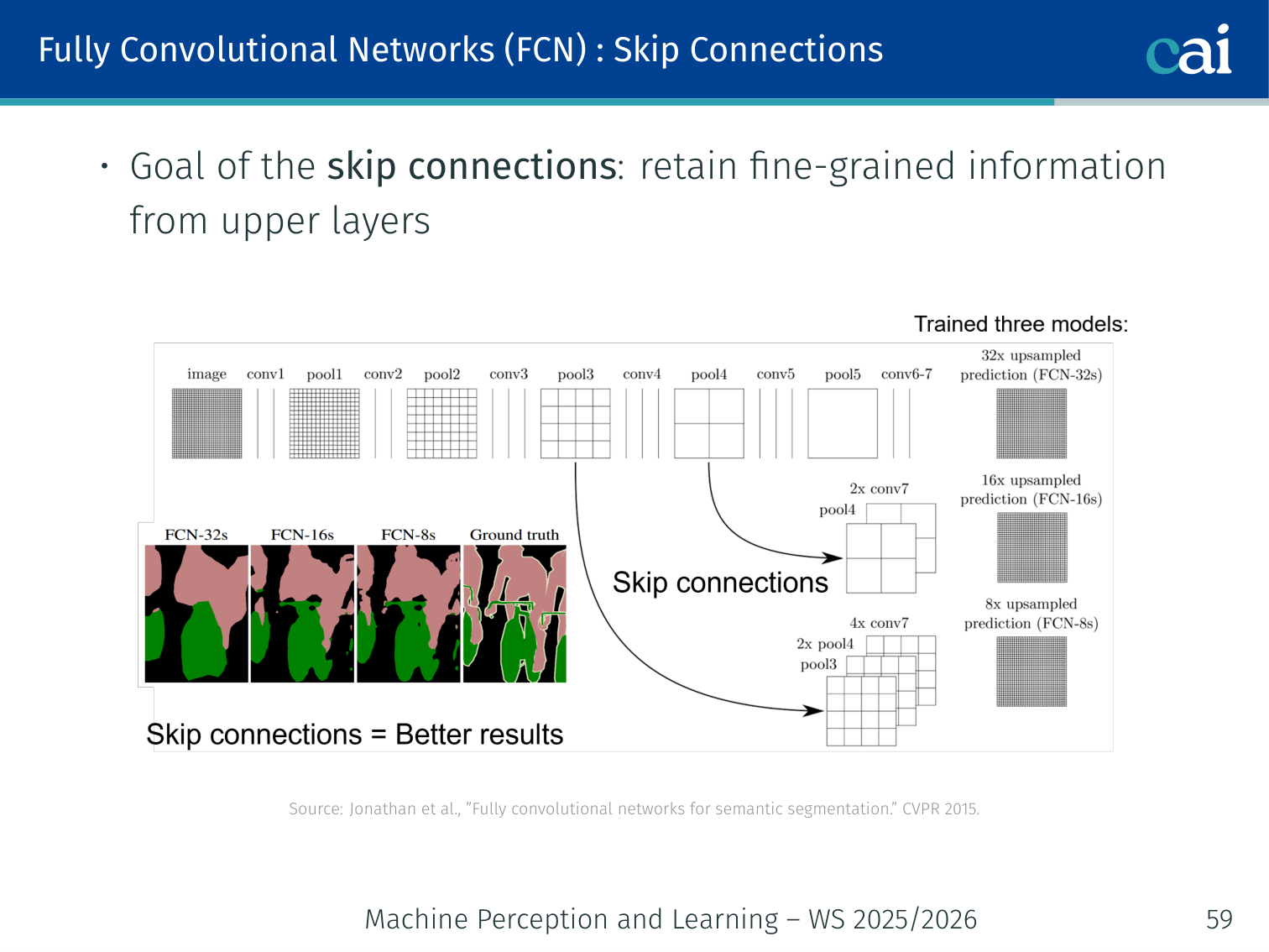
Skip connections combine high-level meaning with low-level detail for sharper masks.

Goal: retain fine-grained spatial information from upper (shallower) layers.

• Coarse deep features carry semantic information; shallow features carry spatial detail
• Skip connections sum predictions from different depths before the final upsampling
• FCN-32s (single upsampling) < FCN-16s (one skip) < FCN-8s (two skips) in quality

Example: the FCN-8s model adds the pool3 prediction (fine spatial detail) to the pool4 prediction, then to the stride-32 prediction before the final 8× upsample — recovering sharper boundary detail than 32× upsampling alone.

---

U-Net [Ronneberger et al., 2015]

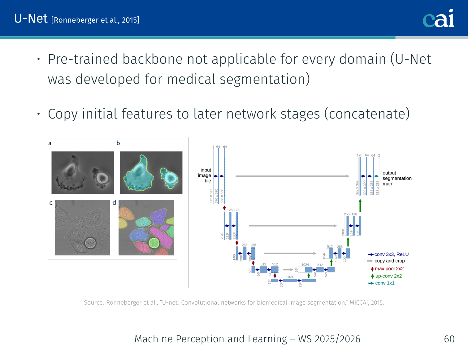
U-Net: the go-to architecture for medical imaging, using "concatenating" skip connections.

• Pre-trained backbone not applicable for every domain (U-Net was developed for medical image segmentation)
• Copies initial features to later network stages (concatenation, not addition)

Encoder (contracting path):       Decoder (expanding path):
Conv → ReLU → MaxPool ──────────→ UpConv + [concatenate] → Conv
Conv → ReLU → MaxPool ──────────→ UpConv + [concatenate] → Conv
         (bottleneck)

• The encoder progressively reduces spatial size and increases channels (captures context)
• The decoder progressively restores spatial size, using concatenated encoder features for precise localisation
• Designed for settings with very limited training data (biomedical imaging)

Example: in retinal vessel segmentation, the encoder path may halve spatial dims 4 times (from 572×572 to 36×36), while the decoder restores back to 388×388, concatenating high-res encoder activations at each step so the output mask retains vessel boundary detail.

---

Mask R-CNN [He et al., 2017]

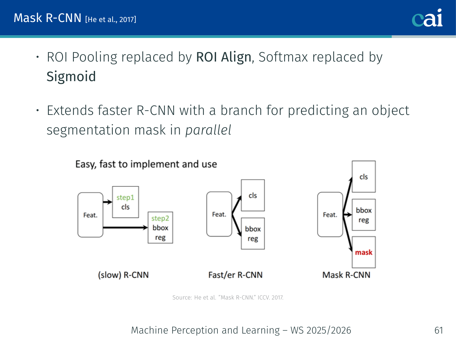
An overview of Mask R-CNN's parallel heads for boxes, classes, and masks.

Extends Faster R-CNN with a branch for predicting an object segmentation mask in parallel with classification and box regression.

Architecture changes:

1. ROI Align replaces ROI Pooling (see below)
2. Softmax replaced by Sigmoid for the mask branch
3. Added mask head predicting a binary mask per class

Loss:

$L=L_{\text{cls}}+L_{\text{box}}+L_{\text{mask}}$

• $L_{\text{cls}}$: sigmoid cross-entropy for classification
• $L_{\text{box}}$: difference between ground truth and output coordinates
• $L_{\text{mask}}$: sigmoid cross-entropy between ground truth binary mask and prediction (not softmax — classes compete only via classification, not through the mask)

The qualitative Mask R-CNN result slide makes the distinction from semantic segmentation concrete: in sports, retail, and beach scenes, the model outputs separate masks for different people or objects of the same class, while keeping the masks aligned to object boundaries. That is the defining extra capability beyond “label every pixel as person/chair/umbrella”.

---

ROI Pooling vs. ROI Align

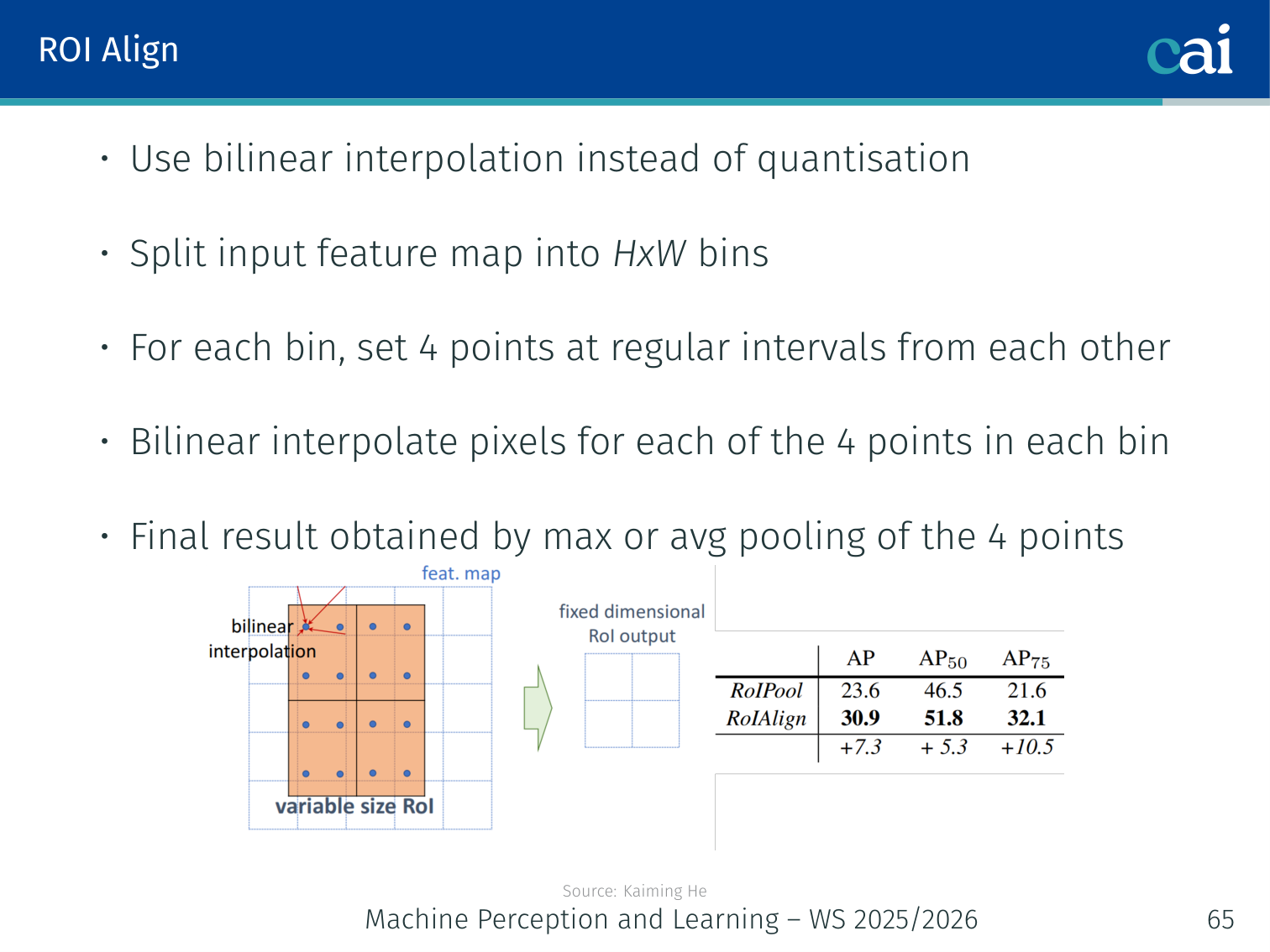
Comparing RoI Pooling and RoI Align: why sub-pixel accuracy matters for masks.

ROI Pooling problem: the CNN predicts floating-point coordinates $(x,y,w,h)$. ROI Pooling must quantise these to integers → introduces pixel misalignment, which breaks accurate segmentation.

ROI Align solution:

• Split the input feature map region into $H\times W$ bins
• For each bin, set 4 sample points at regular subpixel intervals
• Bilinear interpolate the feature values at each of the 4 points
• Max or average pool the 4 points to get the bin value

Example: a proposal at $(10.7,20.3,5.6,8.2)$ would be rounded to $(11,20,6,8)$ in ROI Pooling, introducing quantisation error. ROI Align samples at the exact floating-point coordinates using bilinear interpolation, preserving pixel-to-pixel alignment — critical for mask quality.

	ROI Pooling	ROI Align
Coordinates	Rounded to integers	Floating-point
Alignment error	Present (quantisation)	Eliminated (bilinear interp.)
Segmentation quality	Coarse	Precise

---

Take-Home Messages

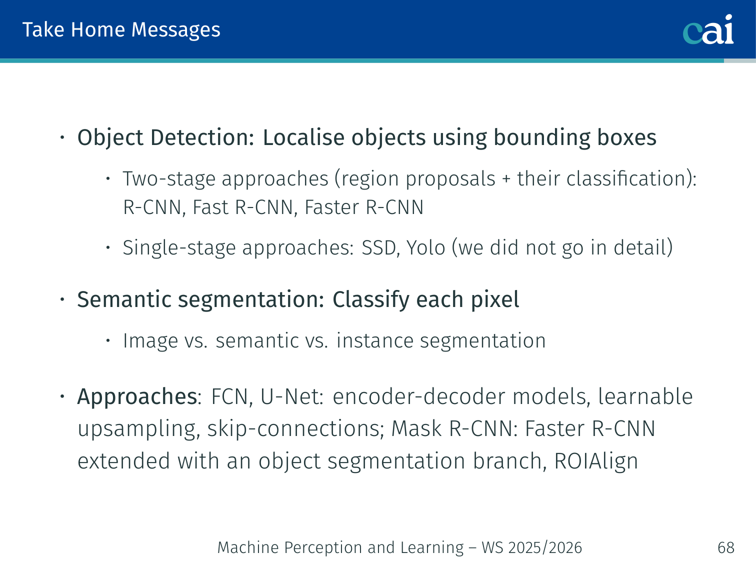
A quick wrap-up of the main methods for detection and segmentation.

• Object Detection: localise objects using bounding boxes
• Two-stage approaches (region proposals + classification): R-CNN → Fast R-CNN → Faster R-CNN
• Single-stage approaches: SSD, YOLO (faster, at some cost in accuracy)
• Semantic segmentation: classify each pixel (no instance distinction); instance segmentation additionally separates same-class objects
• FCN, U-Net: encoder–decoder models with learnable upsampling and skip connections
• Mask R-CNN: Faster R-CNN extended with an object segmentation branch + ROI Align

PyTorch Implementation: ResNet

ResNet uses skip connections to allow training of very deep networks. Below is an implementation of a Residual Block, the fundamental building block of ResNet.

import torch
import torch.nn as nn
import torch.nn.functional as F
 
class ResidualBlock(nn.Module):
    def __init__(self, in_channels, out_channels, stride=1):
        """
        Args:
            in_channels: Number of input feature maps
            out_channels: Number of output feature maps
            stride: Stride for the first convolution (used for downsampling)
        """
        super().__init__()
 
        # --- MAIN PATH ---
        # First 3x3 convolution
        self.conv1 = nn.Conv2d(in_channels, out_channels, kernel_size=3,
                               stride=stride, padding=1, bias=False)
        self.bn1 = nn.BatchNorm2d(out_channels)
 
        # Second 3x3 convolution
        self.conv2 = nn.Conv2d(out_channels, out_channels, kernel_size=3,
                               stride=1, padding=1, bias=False)
        self.bn2 = nn.BatchNorm2d(out_channels)
 
        # --- SKIP CONNECTION (Shortcut) ---
        self.shortcut = nn.Sequential()
 
        # If the input shape doesn't match the output (due to stride or channels),
        # we apply a 1x1 convolution to the shortcut path to match dimensions.
        if stride != 1 or in_channels != out_channels:
            self.shortcut = nn.Sequential(
                nn.Conv2d(in_channels, out_channels, kernel_size=1,
                          stride=stride, bias=False),
                nn.BatchNorm2d(out_channels)
            )
 
    def forward(self, x):
        # 1. Save the input for the identity connection
        identity = self.shortcut(x)
 
        # 2. Compute the main convolutional path
        out = F.relu(self.bn1(self.conv1(x)))
        out = self.bn2(self.conv2(out))
 
        # 3. ADD the identity (residual) to the output
        # This is the "Skip Connection" that allows gradients to flow easily
        out += identity
 
        # 4. Apply final activation after the addition
        return F.relu(out)

Key ResNet Concepts:

• Identity Mapping: By adding the input x to the output $F(x)$, the network only needs to learn the “residual” difference. If a layer isn’t needed, it can easily learn to set its weights to zero, effectively becoming an identity function.
• Gradient Flow: During backpropagation, the gradient can flow directly through the addition gate back to earlier layers, mitigating the vanishing gradient problem in very deep networks (e.g., ResNet-152).
• nn.BatchNorm2d: Essential for stabilizing the distribution of activations, allowing for higher learning rates and faster convergence.

---

References

• Tan, Le (2019) — EfficientNet: Rethinking model scaling for convolutional neural networks. ICML.

Applied Exam Focus

• AlexNet: Key for introducing ReLU and Dropout to scale deep learning.
• VGG: Demonstrated that stacking small $3\times 3$ filters is more efficient than using fewer large filters (e.g., $7\times 7$), as it adds more non-linearities with fewer parameters.
• ResNet: Solved the degradation problem in very deep networks using Skip Connections (Residual blocks), allowing gradients to flow unimpeded.

---

Previous: L02 — CNNs | Back to MPL Index | Next: (y-04) RNNs | (y) Return to Notes | (y) Return to Home