L04 — Recurrent Neural Networks

Previous: L03 — Vision CNNs | Back to MPL Index | Next: (y-05) Transformers

This lecture covers:

• Recurrent Neural Networks
• Backpropagation Through Time
• An Example Task (Image Captioning)
• Long Short-Term Memory (LSTM)

---

Mental Model First

• RNNs are designed for data that arrives as a sequence, where earlier inputs can matter later.
• The hidden state is best viewed as a running summary or working memory that gets updated at each timestep.
• The main challenge is not defining the recurrence, but training it over long horizons without losing useful gradient signal.
• If one question guides this lecture, let it be: how can a model remember enough of the past to make a good decision now?

RNNs — Flexibility in Architecture

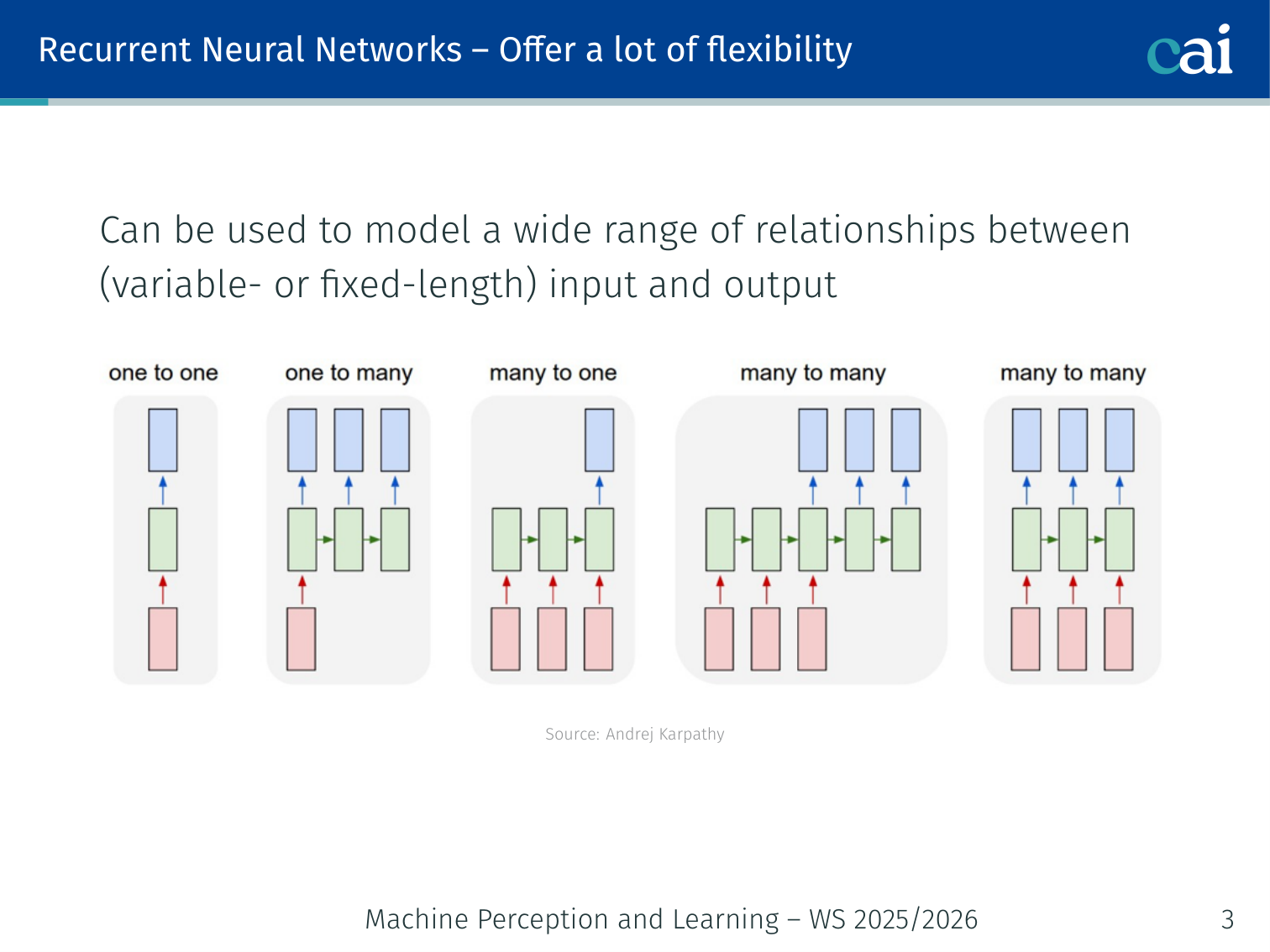
RNNs are super flexible—you can map one or many inputs to one or many outputs.

Unlike feedforward networks, RNNs can model a wide range of relationships between variable- or fixed-length inputs and outputs. The architecture adapts to the task structure.

Type	Input → Output	Example
One-to-one	Fixed → Fixed	Image classification (vanilla NN)
One-to-many	Fixed → Sequence	Image captioning
Many-to-one	Sequence → Fixed	Sentiment classification
Many-to-many (sync)	Sequence → Sequence (aligned)	Video frame labeling
Many-to-many (async)	Sequence → Sequence	Machine translation

---

One-to-One: Vanilla Neural Networks

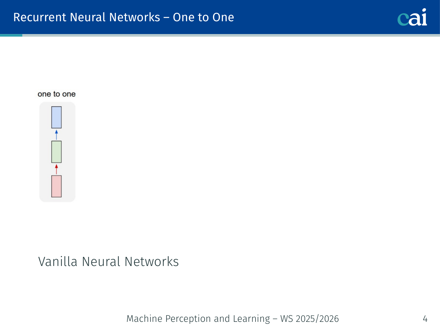
A standard one-to-one setup, just like a classic feedforward network.

A standard feedforward network — one fixed input, one fixed output. The classic example is ImageNet classification (Russakovsky et al., 2015): a single image in, a single class label out.

---

One-to-Many: Image Captioning

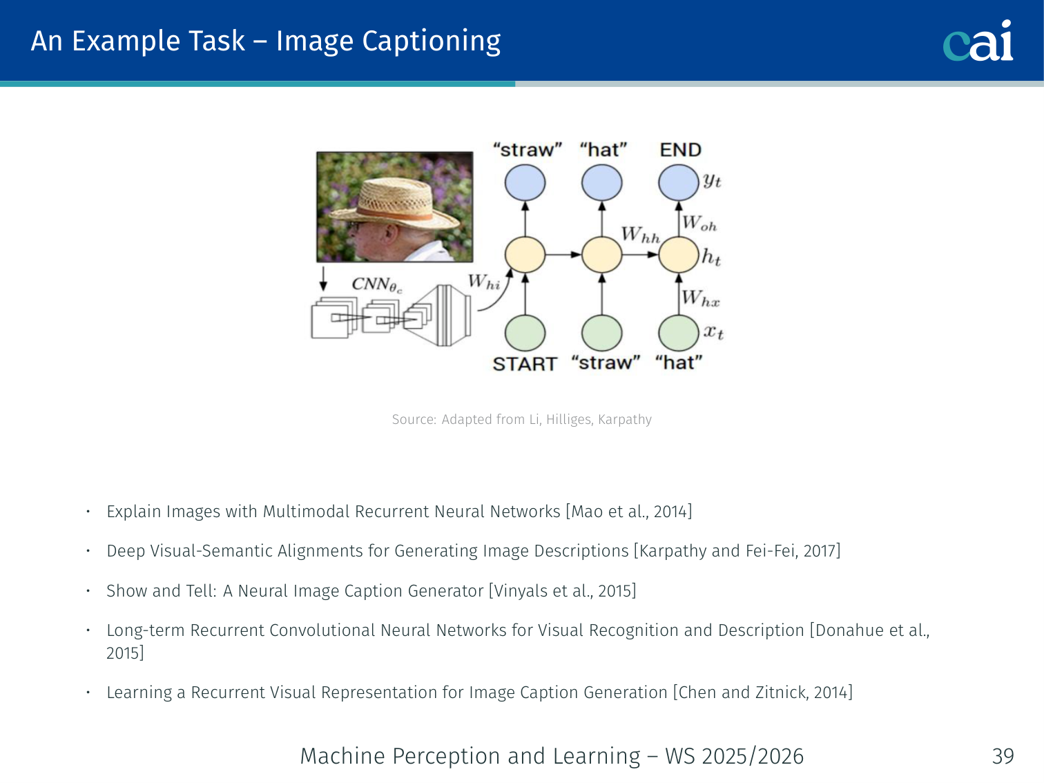
Image captioning is a classic one-to-many problem: one image in, a whole sentence out.

A single fixed-size input (an image) is used to initialize the hidden state of an RNN that then produces a variable-length output sequence (a caption).

Image → h_0 → [RNN] → "A" → [RNN] → "dog" → [RNN] → "on" → [RNN] → "the" → [RNN] → "beach"

Key papers: [Mao et al., 2014], [Vinyals et al., 2015 — “Show and Tell”], [Karpathy & Fei-Fei, 2017], [Donahue et al., 2015], [Chen & Zitnick, 2014]

---

Many-to-One: Sentiment Classification

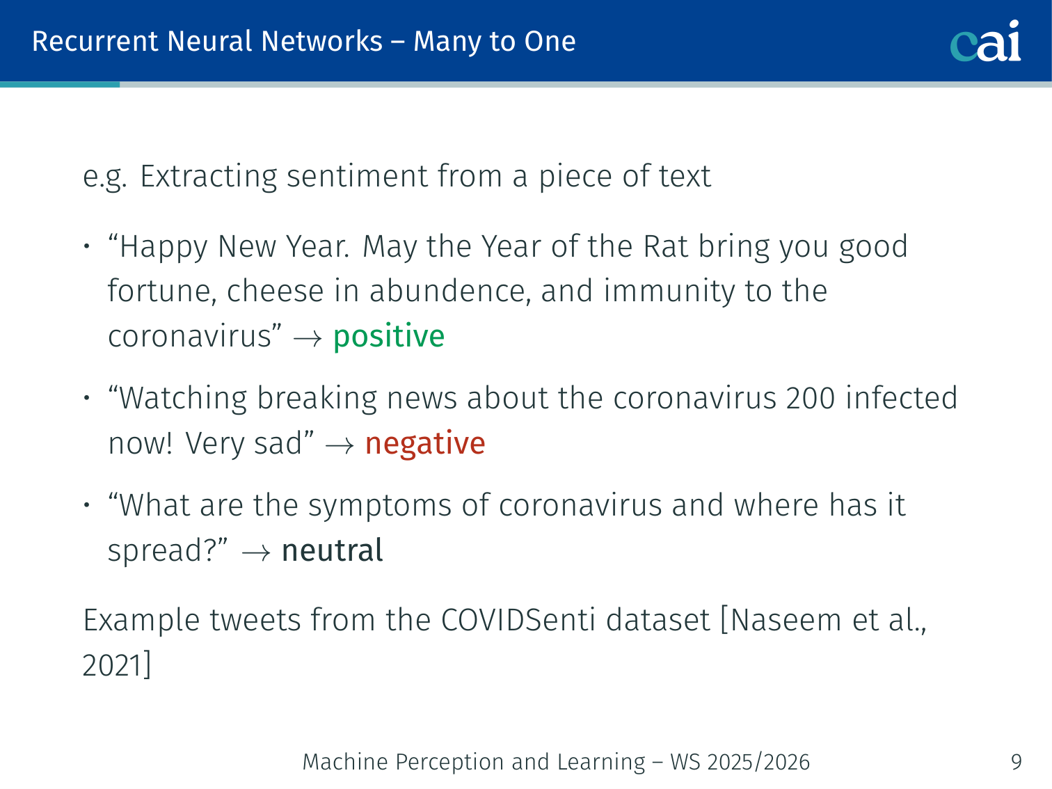
Sentiment analysis takes a full sequence of words and boils it down to a single label.

The entire input sequence is processed step-by-step. The final hidden state summarizes all context from the variable-length input.

Example — COVIDSenti dataset (Naseem et al., 2021):

Tweet	Label
”Happy New Year. May the Year of the Rat bring you good fortune, cheese in abundance…”	Positive
”Watching breaking news about the coronavirus — 200 infected now! Very sad”	Negative
”What are the symptoms of coronavirus and where has it spread?”	Neutral

"Watching" → h_1 → "breaking" → h_2 → ... → "sad" → h_n → [Dense] → Negative

---

Many-to-Many (Sync): Video Classification

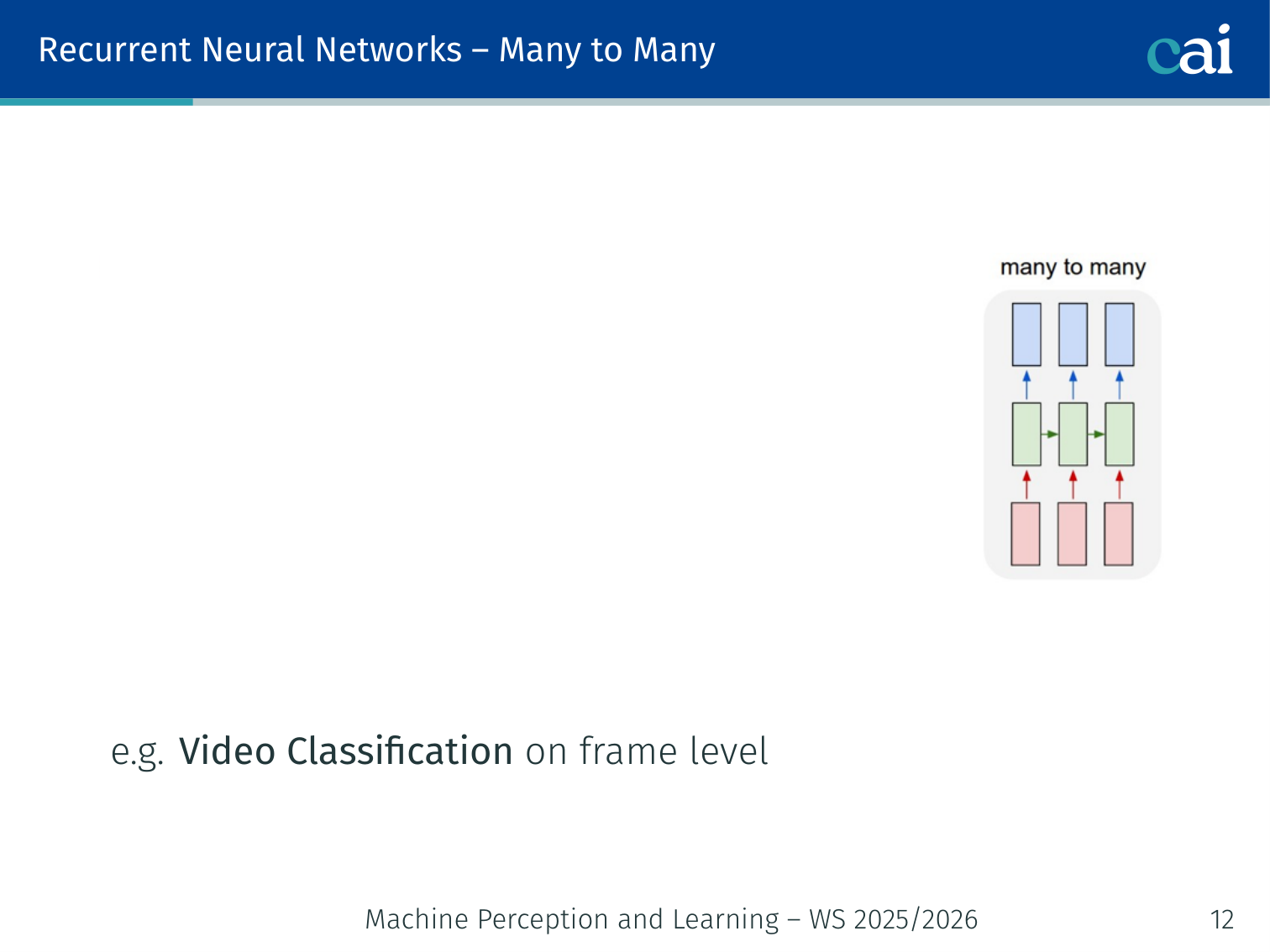
In synchronous many-to-many, the model labels every single frame of a video as it goes.

An output is produced at every time step, aligned with the input. Each frame in a video gets its own label.

Example — Epic-Kitchens dataset (Damen et al., 2018, 2021): First-person video of kitchen activities, with frame-level activity labels (e.g., “chopping”, “stirring”, “pouring”) output at every frame.

---

Many-to-Many (Async): Machine Translation

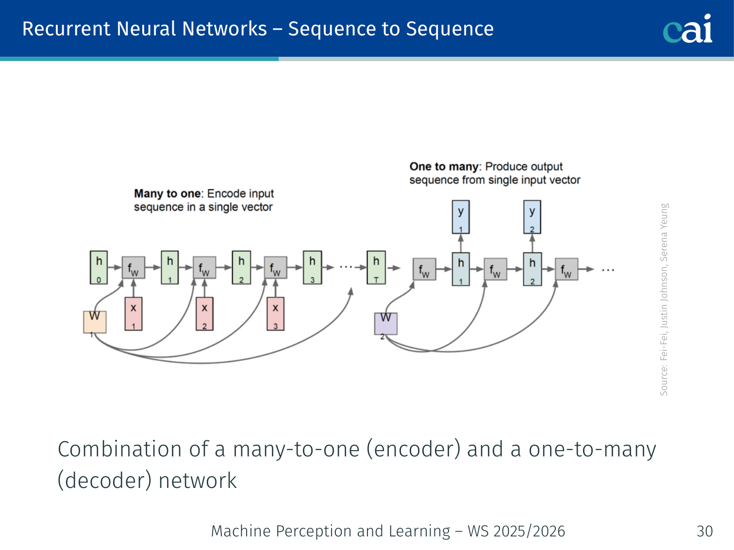
Seq2Seq architectures handle translation by reading the whole sentence before starting to output.

A Sequence-to-Sequence architecture — a combination of:

1. A many-to-one encoder that reads the entire source sentence and compresses it into a context vector
2. A one-to-many decoder that generates the target sentence from that context vector

Example — Google’s Neural Machine Translation (Wu et al., 2016):

Encoder: "I love Paris" → context vector c
Decoder: c → "J'" → "adore" → "Paris"

The final hidden state of the encoder “summarizes” the entire variable-sized input sequence, which then initializes the decoder.

---

The Vanilla RNN — How It Works

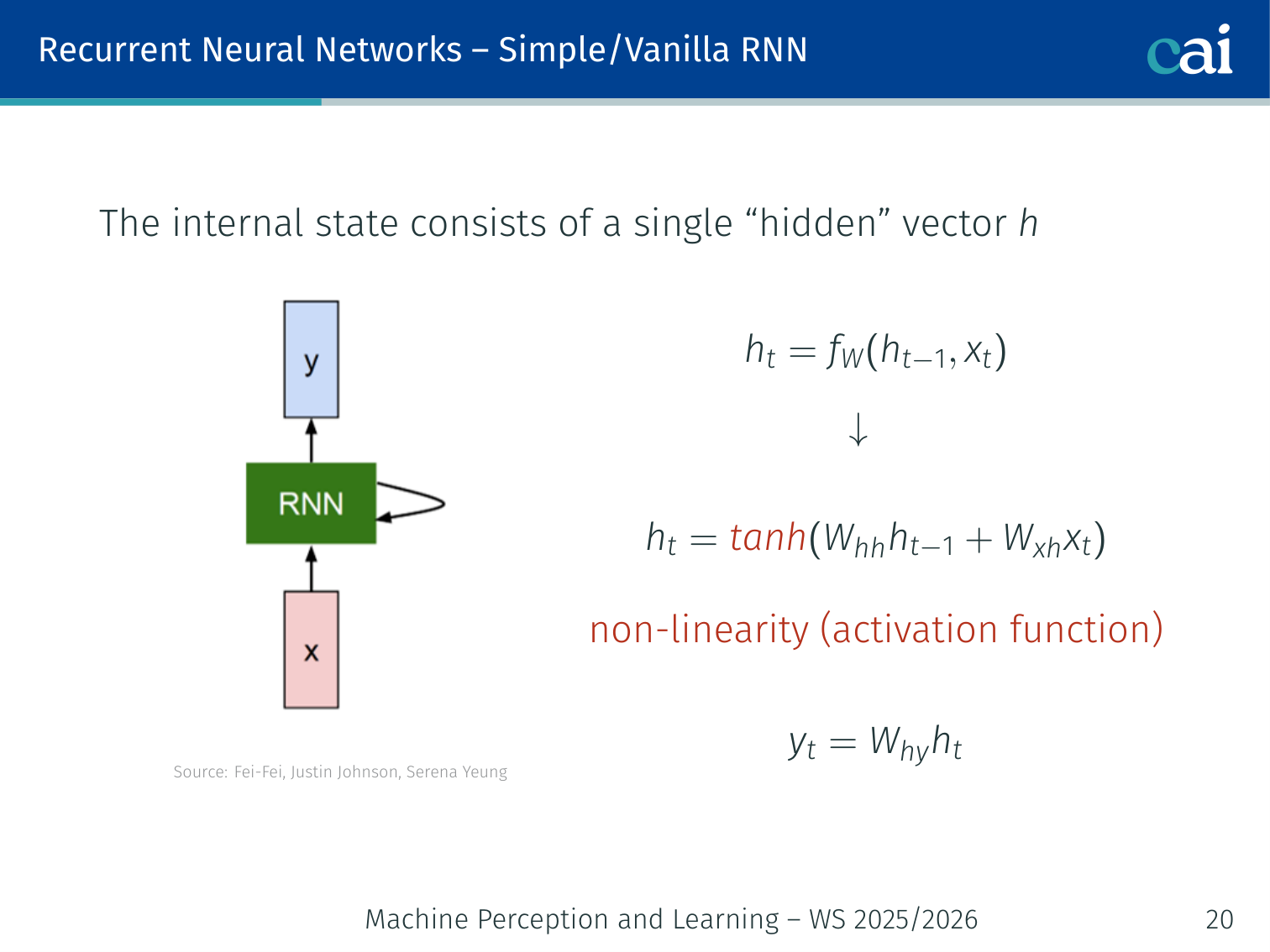
A vanilla RNN uses its hidden state to keep a running memory of what it's seen.

The internal state of a vanilla RNN is a single hidden vector $h$. At each time step $t$:

$h_t=f_W(h_{t-1},x_t)$

More concretely, with a $\tanh$ non-linearity:

$h_t=\tanh (W_{hh}{h}_{t-1}+W_{xh}{x}_t)$

$y_t=W_{hy}{h}_t$

Critical property: At every time step, the input to $f$ is a unique $h_{t-1}$ and $x_t$, but the same weight matrix $W$ is reused at every step. This is parameter sharing across time.

Character-Level Language Model (Karpathy)

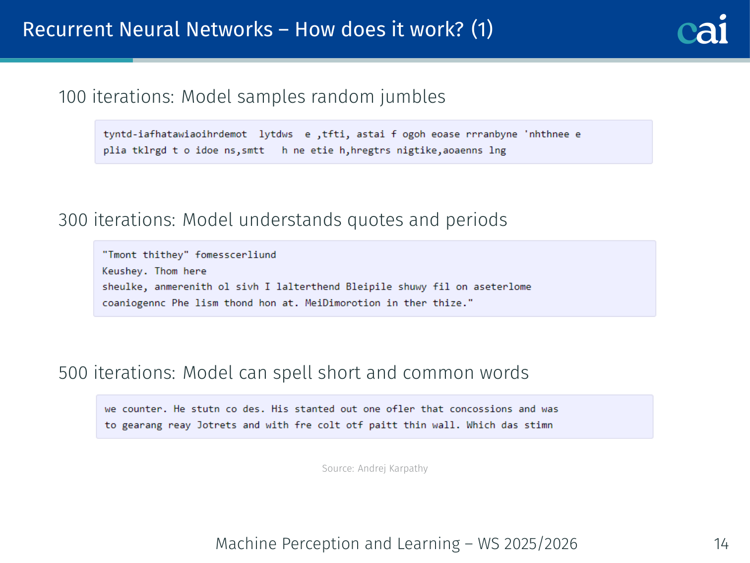
This model predicts the very next character based on everything it's read so far.

Andrej Karpathy’s famous experiment trained a vanilla RNN character-by-character on text corpora. The progression shows what the model learns over training:

Iterations	What the model produces
100	Random jumbles of characters
300	Understands quotes and periods
500	Can spell short and common words
700	English-like text
1,200	Quotations, questions, exclamation marks
2,000	Properly spelled words, quotations, names

After enough training, the same RNN could generate plausible Wikipedia markup, Shakespeare, and even LaTeX code (with math environments, tables, etc.) — all from just predicting the next character.

---

Computational Graphs

Many-to-Many

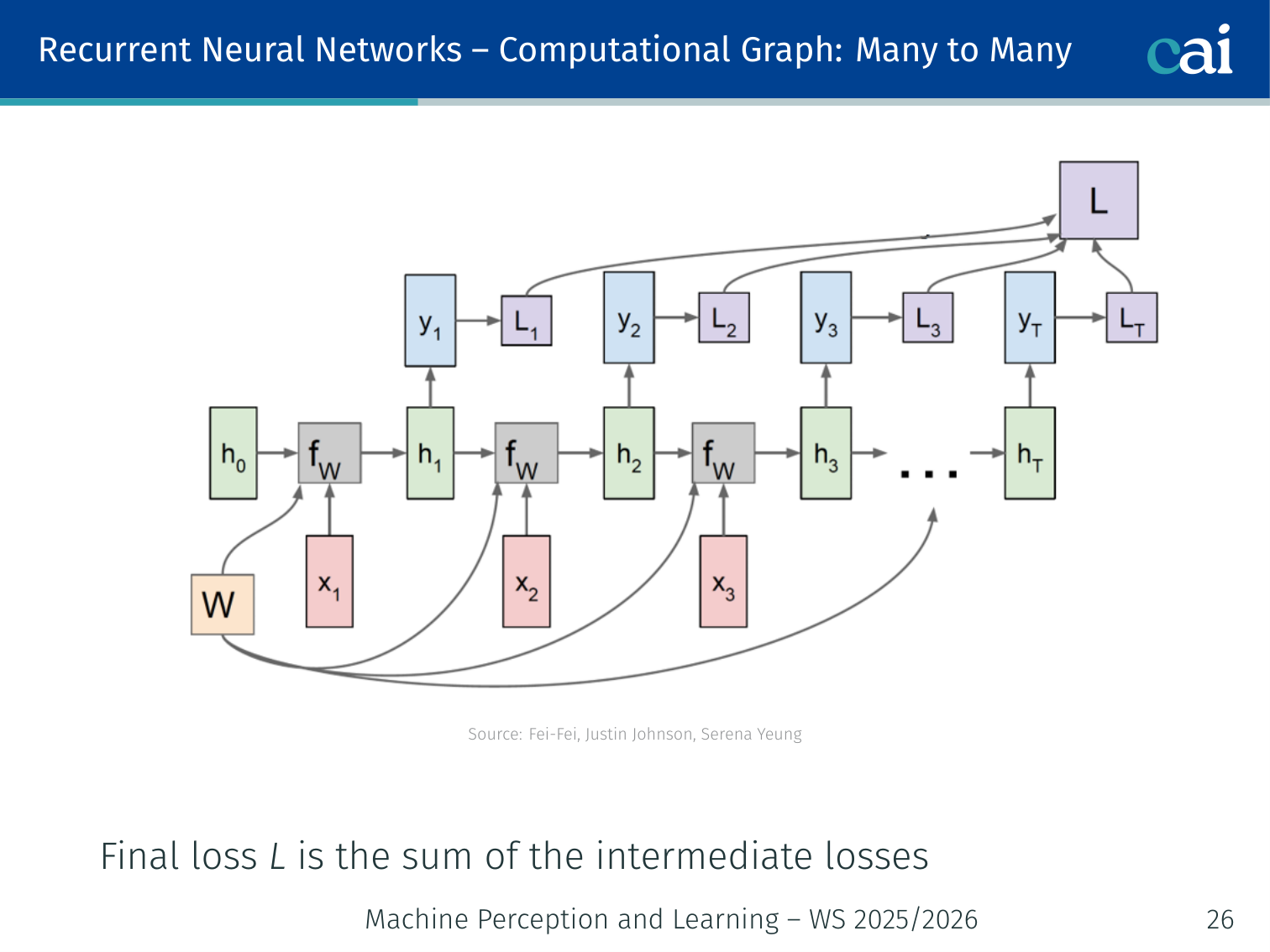
The computational graph for a many-to-many RNN, processing inputs and outputs step-by-step.

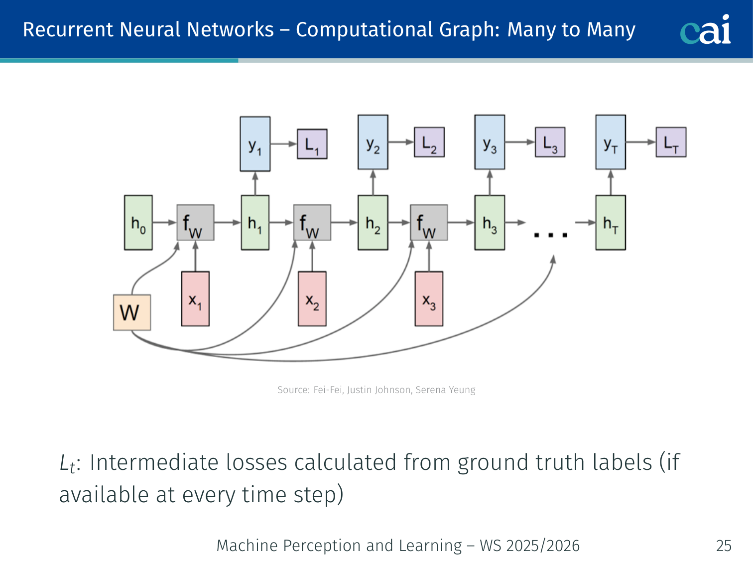
When you unroll the graph, you can see how the loss is calculated at every single timestep.

At every time step $t$, a class score $y_t$ is computed from $h_t$, and an intermediate loss $L_t$ is calculated against ground-truth labels. The final loss $L$ is the sum of all intermediate losses:

$L={\sum }_{t=1}^S{L}_t$

Many-to-One

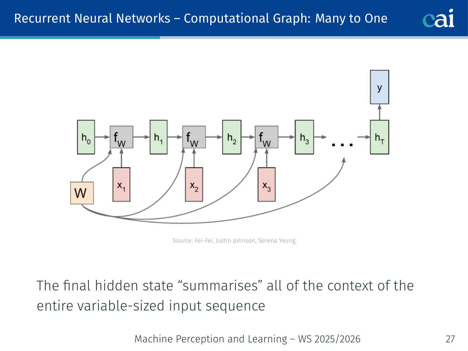
For many-to-one tasks, we only care about the very last output of the sequence.

The network runs through the full sequence but only the final hidden state is used, since it summarizes all prior context.

One-to-Many

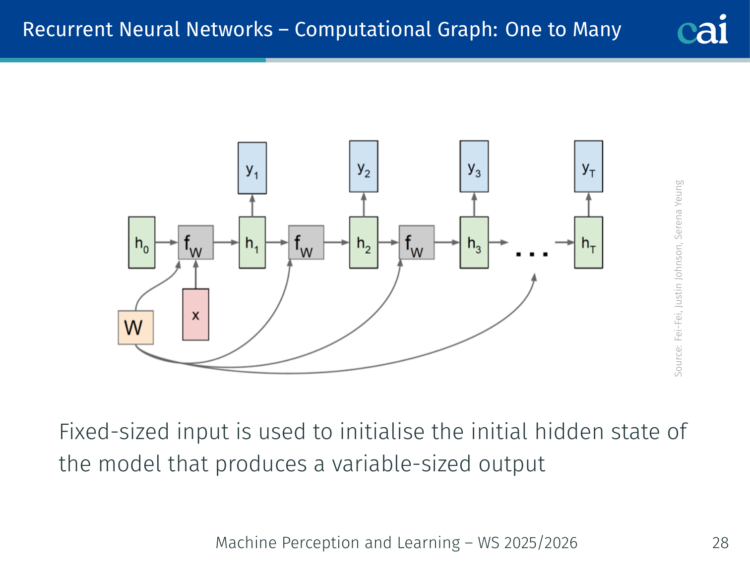
In one-to-many setups, a single initial input kicks off the entire sequence generation.

A fixed-size input (e.g., an image feature vector) initializes $h_0$, and the model then produces a variable-length output.

Sequence-to-Sequence

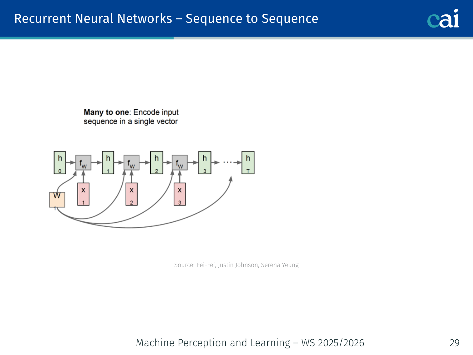
The encoder's job is to read the entire input and compress it into a context vector.

The decoder then takes that context and expands it into a brand new sequence.

Encoder (many-to-one) + Decoder (one-to-many):

x_1 → x_2 → x_3 → [Encoder → c] → y_1 → y_2 → y_3 → y_4

---

Backpropagation Through Time (BPTT)

Intuition

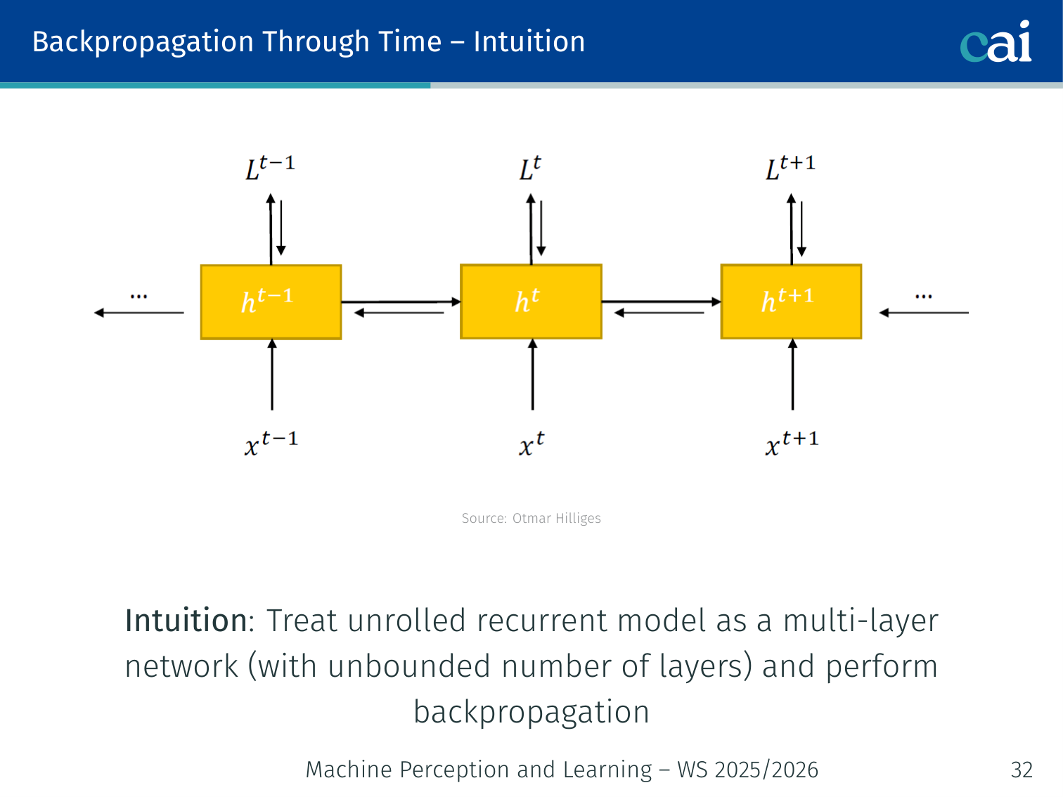
BPTT is basically just regular backprop applied to a network that’s been unrolled across time.

Idea: Treat the unrolled RNN as a multi-layer network with an unbounded number of layers, then apply standard backpropagation through the entire unrolled graph.

The total gradient with respect to $W$ is the sum of the per-timestep gradients:

$\frac{\partial L}{\partial W}={\sum }_{t=1}^S\frac{\partial L_t}{\partial W}$

Each $\frac{\partial L_t}{\partial W}$ requires propagating the error back through all previous time steps.

The Gradient Product

This chain of multiplications is exactly why gradients can get messy in RNNs.

The temporal component that carries error through time is:

$\frac{\partial h_t}{\partial h_k}={\prod }_{i=k+1}^t\frac{\partial h_i}{\partial h_{i-1}}={\prod }_{i=k+1}^t{W}_{hh}^T\cdot \text{diag}({\sigma }^{\prime }(h_{i-1}))$

This is a product of $t-k$ matrices — and that causes problems.

🧠 Deep Dive: Why do Gradients Vanish?

Think of the backward pass in an RNN as a long game of “Telephone.”

1. The loss is calculated at the very end of the sequence.
2. The gradient (the signal) has to travel backward through every time step to reach the beginning.
3. At each step, the signal is multiplied by the weight matrix $W$.
   • If the values in $W$ are slightly smaller than 1 (specifically, if the largest eigenvalue is < 1), the signal shrinks.
   • By the time the signal travels back 50 or 100 steps, it has been multiplied by a small number 100 times. $0.9^{100}\approx 0.00002$.

The Consequence: The network “forgets” the beginning of the sentence because the learning signal never makes it back that far. It can’t learn that a word at step 1 affects a word at step 100.

---

Vanishing Gradients

When gradients vanish, the signal gets so weak that the model completely forgets the start of the sequence.

You can see how the gradient norm drops off fast, making long-term learning almost impossible.

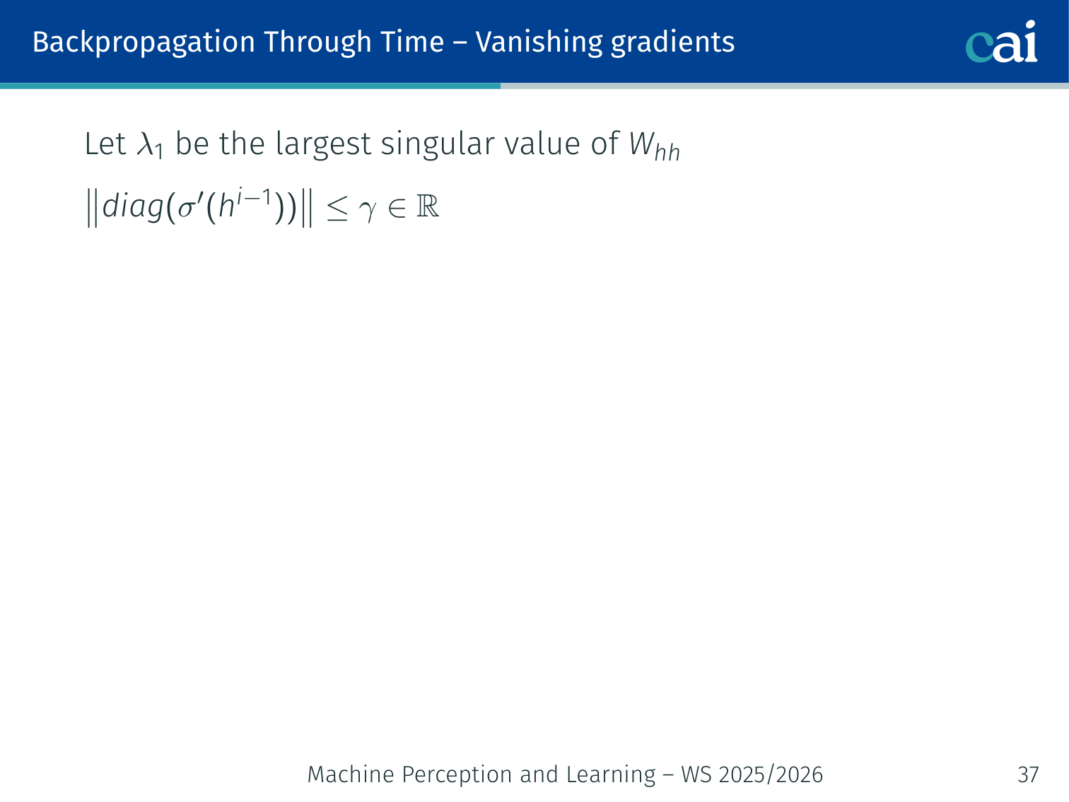
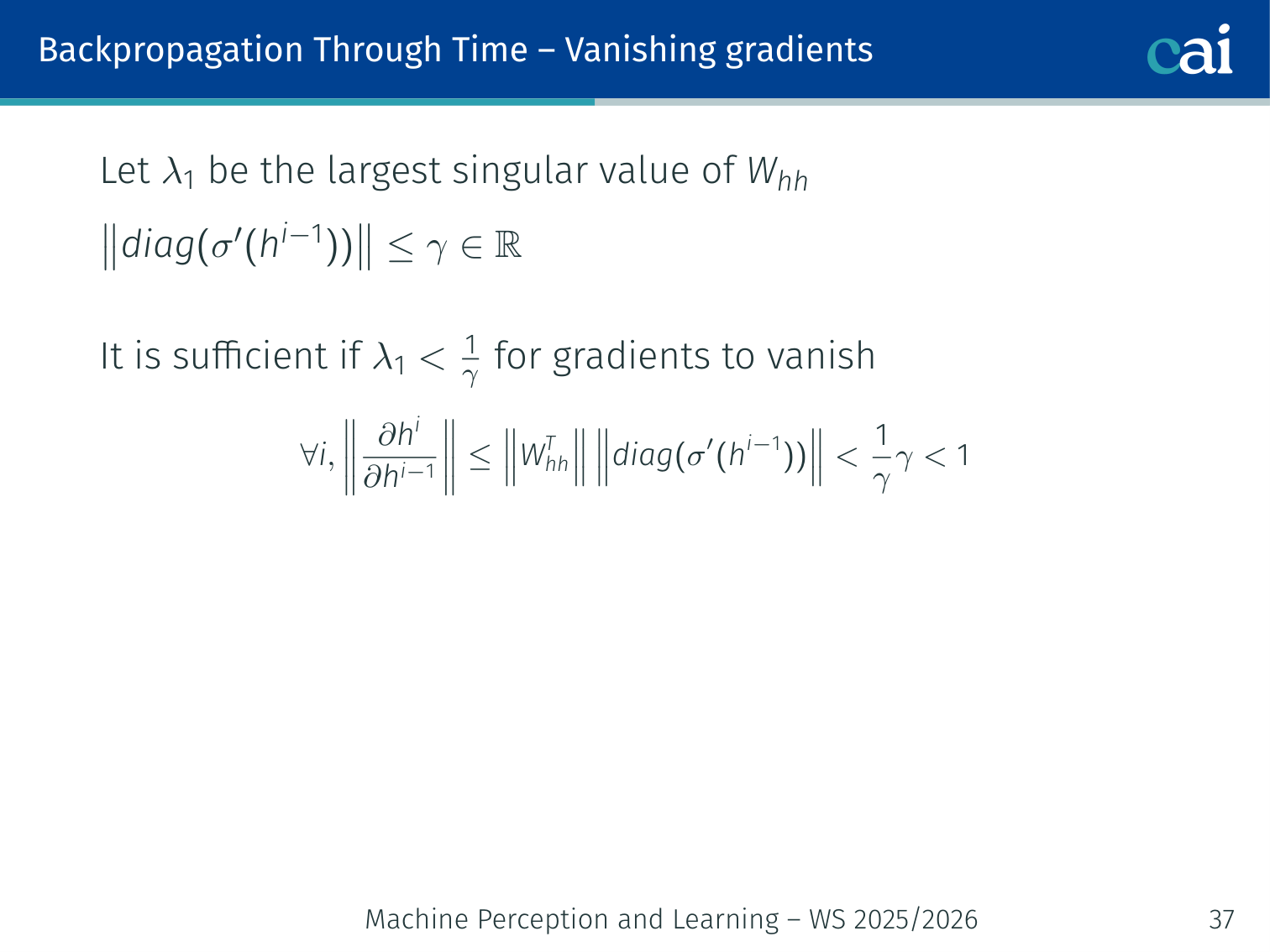
Let ${\lambda }_1$ be the largest singular value of $W_{hh}$.

Theorem: If ${\lambda }_1<\frac{1}{\gamma }$ (where $\gamma$ bounds the derivative of the activation), then:

$\Vert {\prod }_{i=k+1}^t\frac{\partial h_i}{\partial h_{i-1}}\Vert \le {\eta }^{(t-k)}\to 0\text{ as }t-k\to \infty$

Intuitively: if the repeated matrix multiplication shrinks vectors (eigenvalues < 1), gradients vanish exponentially with sequence length. The network cannot learn dependencies between tokens far apart in the sequence.

Eigenvalue intuition: With a linear model $h_t=W^T{h}_{t-1}$, after many steps $h_t=(W^t{)}^T{h}_0$. If $W=Q\Lambda Q^T$, then $h_t=Q^T{\Lambda }^{t}Q\cdot h_0$ — components along eigenvectors with $|\lambda |<1$ vanish, components with $|\lambda |>1$ explode.

Exploding Gradients

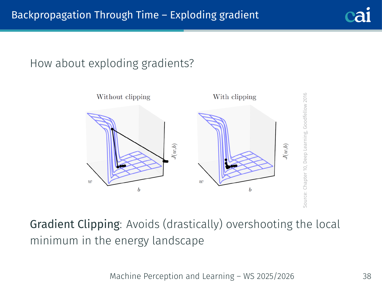
If gradients explode, the updates become so huge that the model's training just falls apart.

The symmetric problem: if ${\lambda }_1>\frac{1}{\gamma }$, gradients grow exponentially, causing drastic overshooting in the loss landscape.

Fix: Gradient Clipping — rescale the gradient vector if its norm exceeds a threshold:

# PyTorch
torch.nn.utils.clip_grad_norm_(model.parameters(), max_norm=1.0)
 
# Equivalent manually
total_norm = sum(p.grad.norm()**2 for p in model.parameters())**0.5
if total_norm > max_norm:
    for p in model.parameters():
        p.grad *= max_norm / total_norm

Gradient clipping prevents overshooting the local minimum in the energy landscape without changing the gradient direction, just its magnitude.

---

Example Task: Image Captioning

Papers

These are the key papers that really kicked off neural image captioning.

• Explain Images with Multimodal Recurrent Neural Networks — Mao et al., 2014
• Deep Visual-Semantic Alignments for Generating Image Descriptions — Karpathy & Fei-Fei, 2017
• Show and Tell: A Neural Image Caption Generator — Vinyals et al., 2015
• Long-term Recurrent Convolutional Networks — Donahue et al., 2015
• Learning a Recurrent Visual Representation for Image Caption Generation — Chen & Zitnick, 2014

Architecture

1. CNN (e.g., VGG, ResNet) — “parses” the image into a fixed-size feature vector
2. RNN — uses the CNN output to initialize $h_0$ and generates the caption word-by-word

Image → [CNN] → v (image vector)
                 ↓
               h_0 = v
               h_1 = tanh(W_hh * h_0 + W_xh * <START>)  → y_1 = "A"
               h_2 = tanh(W_hh * h_1 + W_xh * "A")       → y_2 = "dog"
               h_3 = tanh(W_hh * h_2 + W_xh * "dog")     → y_3 = "on"
               ...                                         → y_n = <END>

Generating Words

At each step, the RNN computes a distribution over all words in the vocabulary (via a softmax over $y_t=W_{hy}{h}_t$), then samples from that distribution. Training maximizes the log-probability of the correct next word at each step.

Code: Minimal Image Captioning RNN

import torch
import torch.nn as nn
import torchvision.models as models
 
class ImageCaptionRNN(nn.Module):
    def __init__(self, embed_dim, hidden_dim, vocab_size):
        super().__init__()
        # CNN encoder (use pretrained ResNet, drop final classifier)
        resnet = models.resnet50(pretrained=True)
        self.cnn = nn.Sequential(*list(resnet.children())[:-1])  # (B, 2048, 1, 1)
        self.cnn_proj = nn.Linear(2048, hidden_dim)
 
        # RNN decoder
        self.embed = nn.Embedding(vocab_size, embed_dim)
        self.rnn = nn.LSTMCell(embed_dim, hidden_dim)
        self.out = nn.Linear(hidden_dim, vocab_size)
 
    def forward(self, image, captions):
        # image: (B, 3, H, W)
        # captions: (B, T) — token ids
        feat = self.cnn(image).squeeze(-1).squeeze(-1)   # (B, 2048)
        h = self.cnn_proj(feat)                           # (B, hidden_dim)
        c = torch.zeros_like(h)
 
        outputs = []
        for t in range(captions.size(1)):
            x = self.embed(captions[:, t])               # (B, embed_dim)
            h, c = self.rnn(x, (h, c))
            logits = self.out(h)                         # (B, vocab_size)
            outputs.append(logits)
 
        return torch.stack(outputs, dim=1)               # (B, T, vocab_size)

---

Long Short-Term Memory (LSTM)

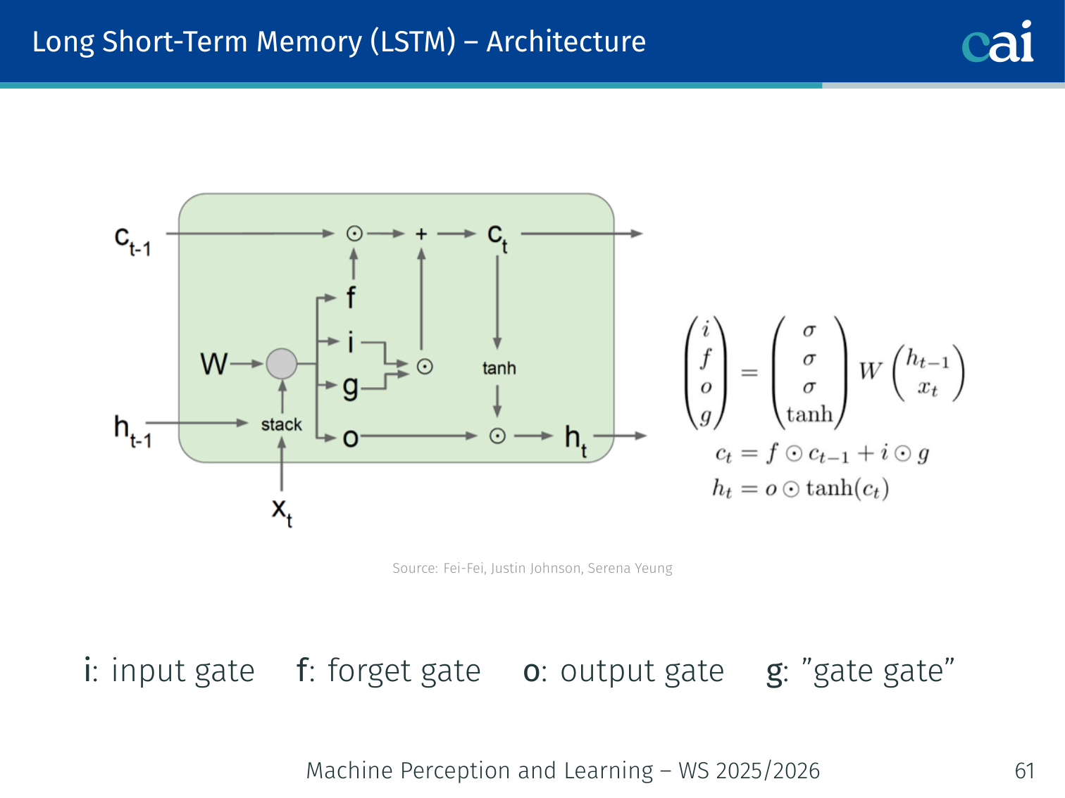
An LSTM adds a cell state and special gates to help information flow much more easily.

The input, forget, and output gates work together to manage what stays in memory.

Authors: Hochreiter & Schmidhuber, 1997

Motivation

Vanilla RNNs fail on long sequences because of vanishing gradients. The fix is to change the RNN architecture to improve gradient flow.

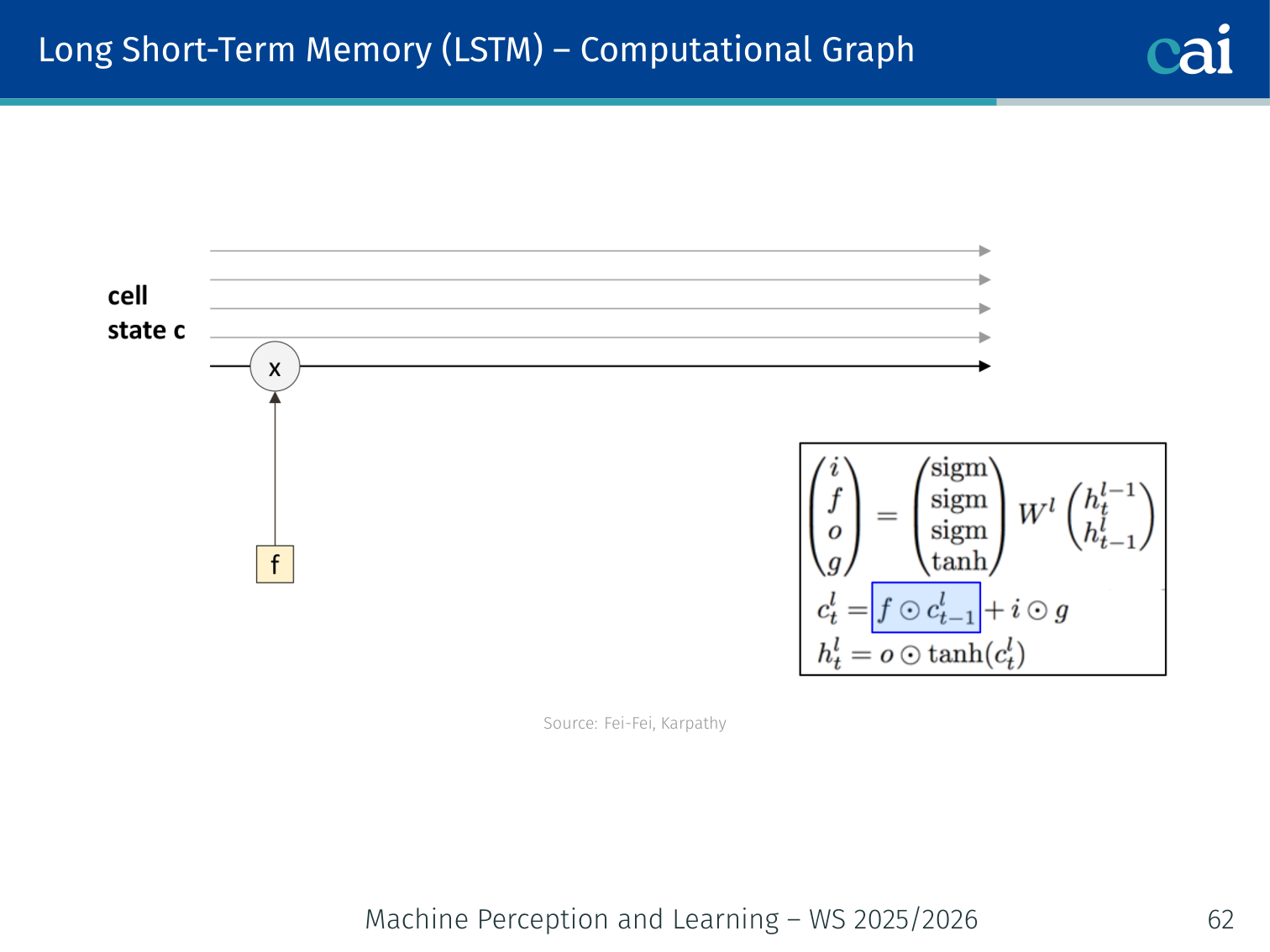
The key idea: introduce a cell state $c_t$ that runs alongside the hidden state $h_t$. The cell state is updated via additive interactions rather than repeated matrix multiplications, giving gradients a highway to flow through.

💡 Intuition: LSTM as a “Managed” Memory

A vanilla RNN is like a notebook where you have to erase the whole page and rewrite it every time you hear a new word. You quickly lose track of what happened at the start.

An LSTM is more like a professional filing system (the Cell State):

• Forget Gate: “Is this old information (e.g., the subject of the previous sentence) still relevant? If not, shred it.”
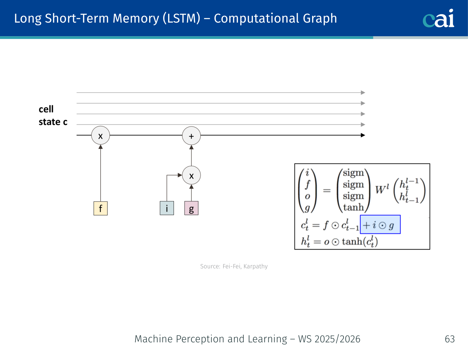
• Input Gate: “Is this new word important enough to write down in our permanent record?”
• Output Gate: “What parts of our internal files should we actually tell the next layer right now?”

Because information can stay in the “files” (Cell State) without being modified, it can travel across hundreds of steps perfectly intact.

---

The Four Gates

These four gates are the "management team" that controls the flow of information through an LSTM.

The LSTM uses four learned gating vectors, all computed from $[h_{t-1},x_t]$:

Gate	Symbol	Role
Input gate	$i$	How much new information to write
Forget gate	$f$	How much old cell state to keep
Output gate	$o$	How much cell state to expose
Gate gate	$g$	Candidate new cell content ($\tanh$ activation)

$\left(\begin{array}{c}i\\ f\\ o\\ g\end{array}\right)=\left(\begin{array}{c}\sigma \\ \sigma \\ \sigma \\ \tanh \end{array}\right)\left(W\left(\begin{array}{c}{h}_{t-1}\\ x_t\end{array}\right)+b\right)$

(In practice, $W$ is a single stacked weight matrix — this is why PyTorch computes all four gates in one matmul.)

Cell State and Hidden State Update

$c_t=f\odot c_{t-1}+i\odot g\text{(additive update)}$ $h_t=o\odot \tanh (c_t)$

where $\odot$ is the Hadamard (element-wise) product.

Intuition — Concrete Example

LSTMs are great at remembering things like subject-verb agreement over long distances.

Parsing: “The cats, which lived in Paris, were ___”

1. Read “cats” → input gate opens, writes “plural subject” into $c_t$
2. Process “which lived in Paris” → forget gate ≈ 1 (keep memory), input gate selectively writes clause info
3. Encounter “were” blank → output gate opens, exposes “plural” from $c_t$
4. Prediction: “were” (not “was”)

A vanilla RNN “forgets” the subject after many steps. The LSTM’s cell state preserves it.

Why Gradient Flow is Better

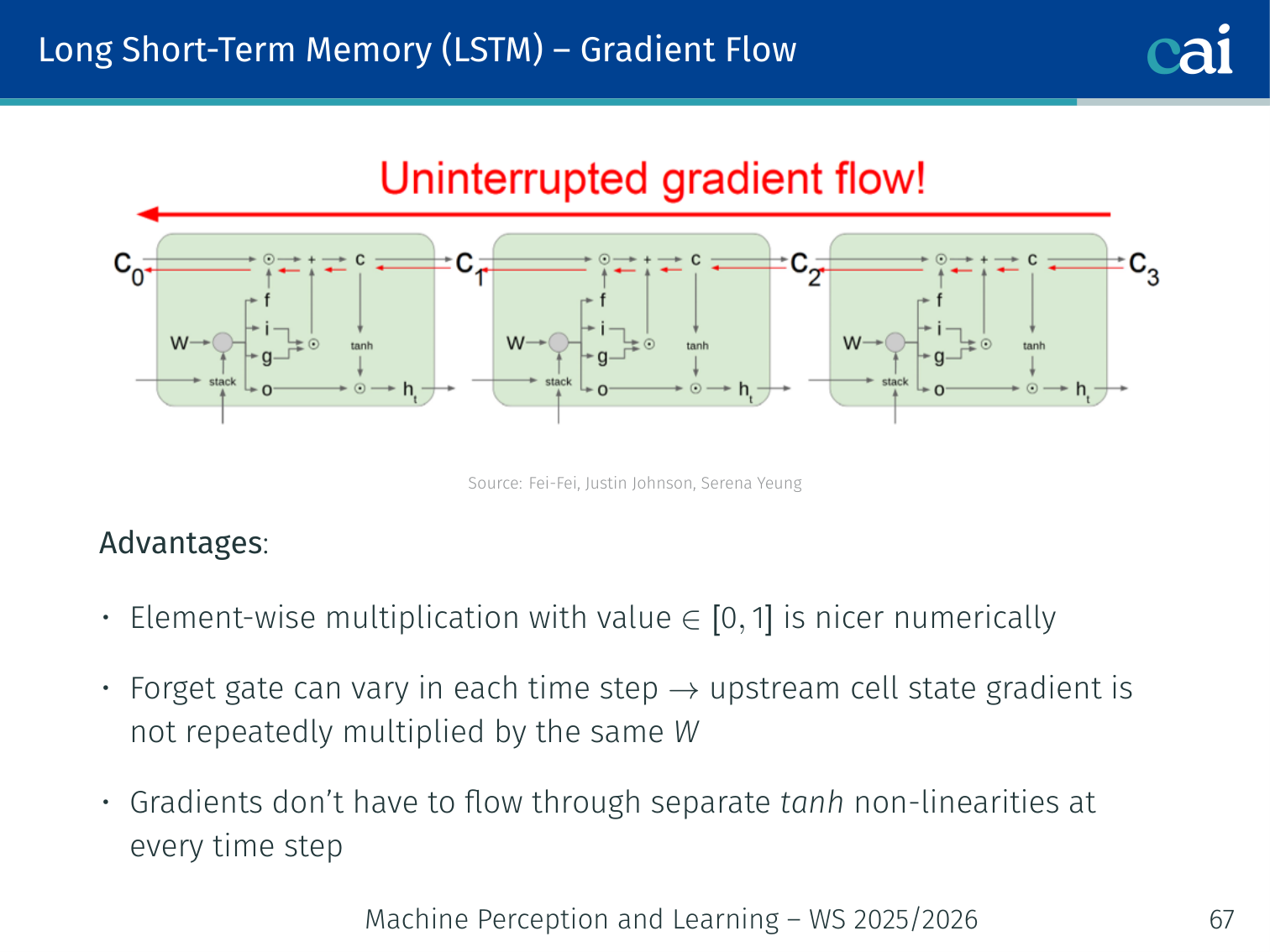
The cell state acts like a highway, letting gradients travel deep into the past without fading.

Three reasons gradients flow more easily through LSTMs (Fei-Fei, Justin Johnson, Serena Yeung):

1. Element-wise multiplication with $f\in [0,1]$ — numerically nicer than multiplying by the full $W_{hh}$ repeatedly. The forget gate attenuates rather than chaotically distorts.

2. Forget gate varies per time step — unlike vanilla RNNs where the same $W$ multiplies at every step (causing exponential behavior), the effective “weight” on $c_{t-1}$ changes each step.

3. No $\tanh$ at every step — gradients flow directly through the additive cell update $c_t=f\odot c_{t-1}+i\odot g$. The $\tanh$ is only applied once at the output, not at every recurrent step.

The cell state $c_t$ is a gradient highway: signals can travel hundreds of time steps with minimal distortion.

Code: LSTM for Sentiment Classification

import torch
import torch.nn as nn
 
class SentimentLSTM(nn.Module):
    def __init__(self, vocab_size, embed_dim, hidden_dim, num_classes, num_layers=2):
        super().__init__()
        self.embed = nn.Embedding(vocab_size, embed_dim, padding_idx=0)
        self.lstm = nn.LSTM(
            embed_dim, hidden_dim,
            num_layers=num_layers,
            batch_first=True,
            dropout=0.3,
            bidirectional=True
        )
        self.classifier = nn.Linear(hidden_dim * 2, num_classes)  # ×2 for bidirectional
        self.dropout = nn.Dropout(0.3)
 
    def forward(self, x):
        # x: (B, T) — token IDs
        emb = self.dropout(self.embed(x))          # (B, T, E)
        out, (h_n, c_n) = self.lstm(emb)           # out: (B, T, H*2)
        # Use the final time step's hidden state
        pooled = out[:, -1, :]                     # (B, H*2)
        return self.classifier(self.dropout(pooled))  # (B, num_classes)
 
# Example: COVIDSenti-style 3-class sentiment
model = SentimentLSTM(vocab_size=30000, embed_dim=128, hidden_dim=256, num_classes=3)
 
# Training step
optimizer = torch.optim.Adam(model.parameters(), lr=1e-3)
criterion = nn.CrossEntropyLoss()
 
# tokens = tokenize("Watching breaking news about the coronavirus...")
# logits = model(tokens)  →  class 1 (Negative)

---

GRU — Gated Recurrent Unit

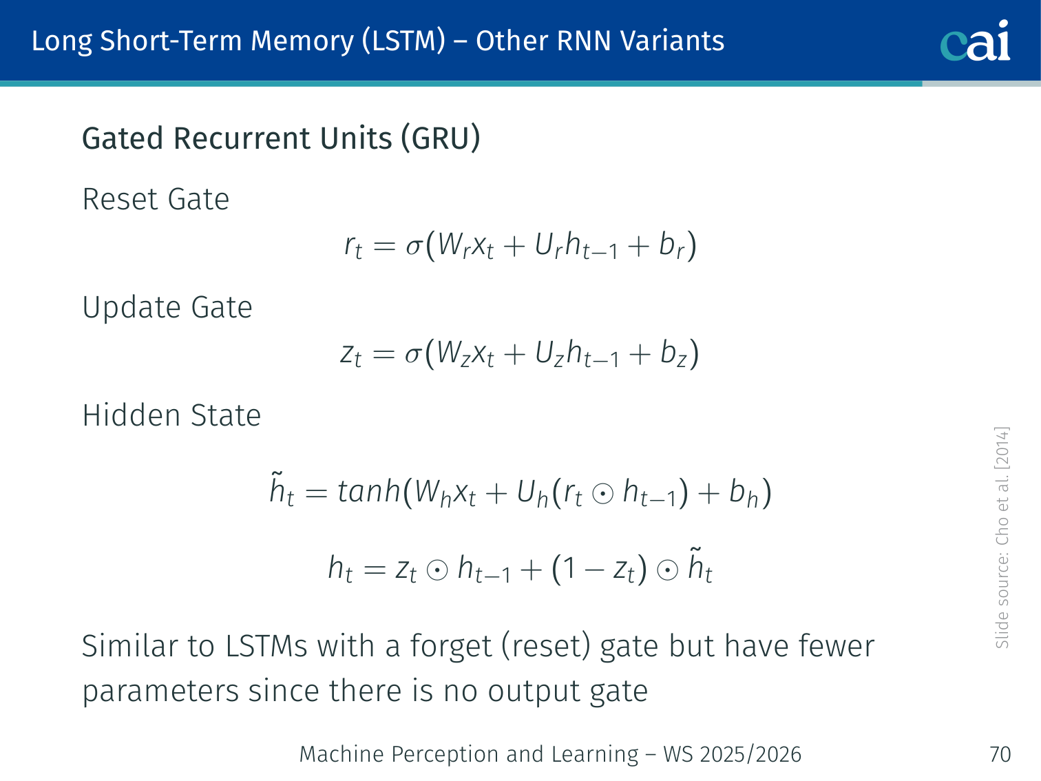
A GRU simplifies things by merging gates and getting rid of the separate cell state.

Authors: Cho et al., 2014

GRU simplifies LSTM by merging the forget and input gates into a single update gate and eliminating the separate cell state. There is no output gate.

$r_t=\sigma (W_r{x}_t+U_r{h}_{t-1}+b_r)\text{(reset gate)}$ $z_t=\sigma (W_z{x}_t+U_z{h}_{t-1}+b_z)\text{(update gate)}$ ${\tilde{h}}_t=\tanh (W_h{x}_t+U_h(r_t\odot h_{t-1})+b_h)\text{(candidate state)}$ $h_t=z_t\odot h_{t-1}+(1-z_t)\odot {\tilde{h}}_t\text{(new hidden state)}$

Reset gate $r_t$: controls how much of the previous hidden state to use when computing the candidate ${\tilde{h}}_t$. When $r_t\approx 0$, the model ignores the past — useful for starting a new segment.

Update gate $z_t$: interpolates between the old hidden state and the candidate. When $z_t\approx 1$, the old state is copied (similar to LSTM’s forget gate ≈ 1).

GRU vs LSTM

Comparing the inner workings of GRUs and LSTMs—one is leaner, the other is more complex.

	GRU	LSTM
Parameters	Fewer (no output gate)	More
States	One ($h_t$)	Two ($h_t$ and $c_t$)
Speed	Faster	Slower
Long sequences	Slightly weaker	Stronger
Practice	Often comparable	Often comparable

Neither always wins. Try both. For tasks where training speed matters and sequences are moderate length, GRU is a good default.

import torch.nn as nn
 
# Drop-in GRU replacement for LSTM
gru = nn.GRU(input_size=128, hidden_size=256, num_layers=2,
             batch_first=True, dropout=0.3, bidirectional=True)

---

Bidirectional LSTM (BiLSTM)

Bidirectional LSTMs get the full picture by looking at the sequence from both ends at once.

Authors: Graves & Schmidhuber, 2005

A standard RNN only uses past context — it cannot see future tokens when processing position $t$. A BiLSTM runs two separate LSTMs over the same sequence:

• Forward pass (left → right): processes $x_1,x_2,\dots ,x_T$
• Backward pass (right → left): processes $x_T,x_{T-1},\dots ,x_1$

The hidden states from both passes are concatenated at each position:

$h_t^{bi}=[\overrightarrow{h_t};\overleftarrow{h_t}]$

Forward Pass Equations

${\overrightarrow{i}}_t=\sigma ({\overrightarrow{W}}_i{x}_t+{\overrightarrow{U}}_i{h}_{t-1}+{\overrightarrow{b}}_i)$ ${\overrightarrow{f}}_t=\sigma ({\overrightarrow{W}}_f{x}_t+{\overrightarrow{U}}_f{h}_{t-1}+{\overrightarrow{b}}_f)$ ${\overrightarrow{o}}_t=\sigma ({\overrightarrow{W}}_o{x}_t+{\overrightarrow{U}}_o{h}_{t-1}+{\overrightarrow{b}}_o)$ ${\overrightarrow{\tilde{c}}}_t=\tanh ({\overrightarrow{W}}_c{x}_t+{\overrightarrow{U}}_c{h}_{t-1}+{\overrightarrow{b}}_c)$ ${\overrightarrow{c}}_t={\overrightarrow{f}}_t\odot {\overrightarrow{c}}_{t-1}+{\overrightarrow{i}}_t\odot {\overrightarrow{\tilde{c}}}_t$ ${\overrightarrow{h}}_t={\overrightarrow{o}}_t\odot \tanh ({\overrightarrow{c}}_t)$

Backward Pass Equations

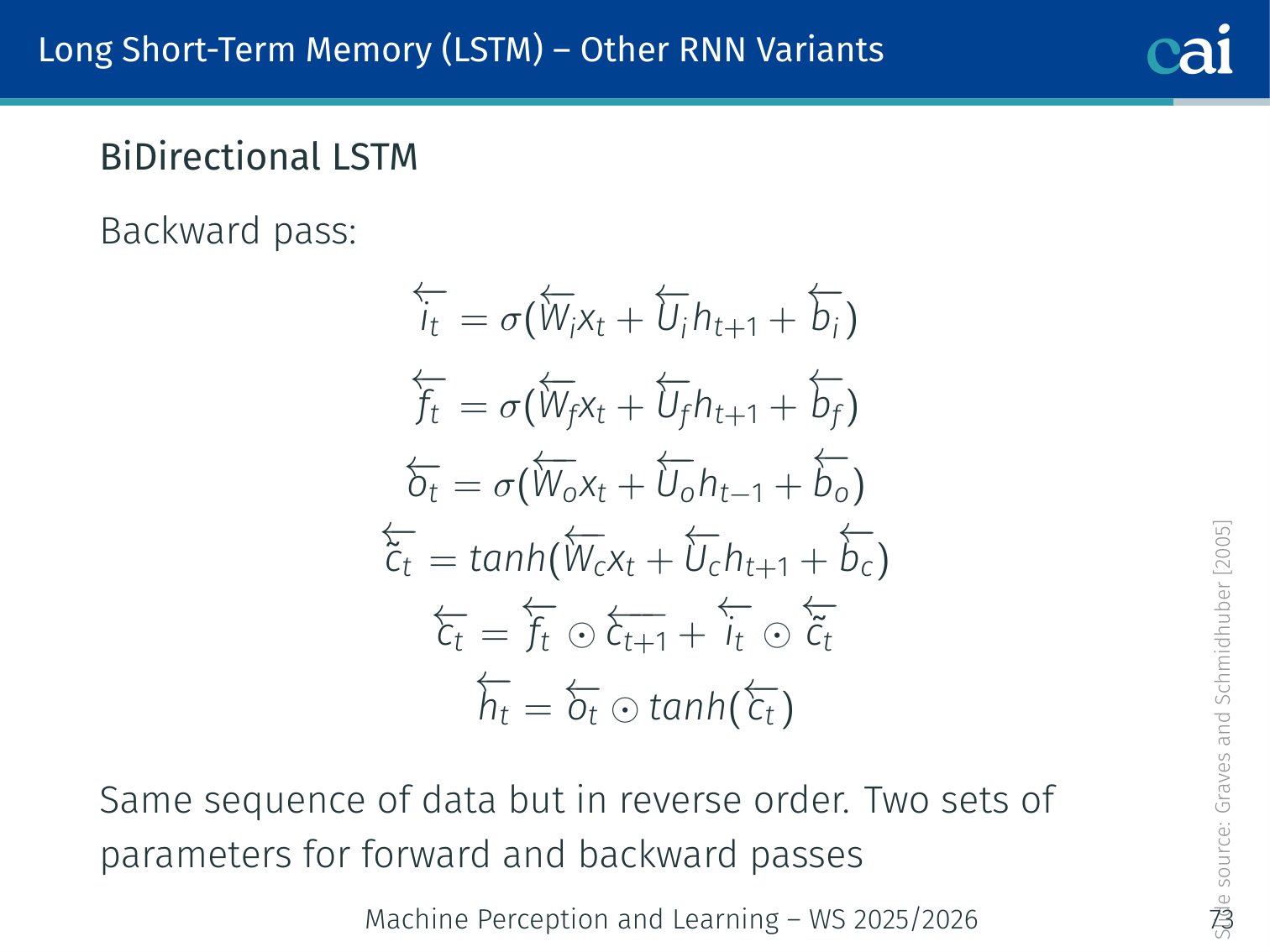
The backward pass uses its own set of parameters to learn from the future context.

Same structure, but indices go from $T$ to $1$ and $h_{t-1}$ is replaced by $h_{t+1}$:

${\overleftarrow{i}}_t=\sigma ({\overleftarrow{W}}_i{x}_t+{\overleftarrow{U}}_i{h}_{t+1}+{\overleftarrow{b}}_i)$ ${\overleftarrow{c}}_t={\overleftarrow{f}}_t\odot {\overleftarrow{c}}_{t+1}+{\overleftarrow{i}}_t\odot {\overleftarrow{\tilde{c}}}_t$ ${\overleftarrow{h}}_t={\overleftarrow{o}}_t\odot \tanh ({\overleftarrow{c}}_t)$

There are two separate sets of parameters — one for each direction.

When to Use BiLSTM

• Yes: any task where the full sequence is available at inference time — text classification, named entity recognition (NER), machine translation encoding
• No: language generation / autoregressive decoding — you can’t look at future tokens you haven’t generated yet

bilstm = nn.LSTM(input_size=128, hidden_size=256,
                 batch_first=True, bidirectional=True)
# Output: (B, T, 512)  — 256 forward + 256 backward

Example: NER with BiLSTM

# Sentence: "Barack Obama was born in Hawaii"
# Each token gets a tag: B-PER, I-PER, O, O, O, B-LOC
 
class BiLSTMNER(nn.Module):
    def __init__(self, vocab_size, embed_dim, hidden_dim, num_tags):
        super().__init__()
        self.embed = nn.Embedding(vocab_size, embed_dim)
        self.bilstm = nn.LSTM(embed_dim, hidden_dim,
                              batch_first=True, bidirectional=True)
        self.fc = nn.Linear(hidden_dim * 2, num_tags)
 
    def forward(self, x):
        emb = self.embed(x)                  # (B, T, E)
        out, _ = self.bilstm(emb)            # (B, T, 2H)
        return self.fc(out)                  # (B, T, num_tags)
 
# Each token in the sentence gets a prediction using both left and right context

PyTorch Implementation: RNN and Seq2Seq

Below is an implementation of a basic Sequence-to-Sequence (Seq2Seq) model, commonly used for tasks like Machine Translation.

import torch
import torch.nn as nn
import torch.nn.functional as F
 
# 1. The ENCODER: reads the source sequence and compresses it
class Encoder(nn.Module):
    def __init__(self, vocab_size, embed_dim, hidden_dim):
        super().__init__()
        # nn.Embedding converts word indices into dense vectors
        self.embedding = nn.Embedding(vocab_size, embed_dim)
 
        # GRU (Gated Recurrent Unit) processes the sequence
        # hidden_dim is the size of the "memory" or context vector
        self.gru = nn.GRU(embed_dim, hidden_dim)
 
    def forward(self, x):
        # x: Input indices of shape (seq_len, batch_size)
        embedded = self.embedding(x)
 
        # output: all hidden states for every step in the sequence
        # hidden: the FINAL hidden state (the "context vector")
        output, hidden = self.gru(embedded)
 
        # We only need the final hidden state to initialize the decoder
        return output, hidden
 
# 2. The DECODER: generates the target sequence one step at a time
class Decoder(nn.Module):
    def __init__(self, vocab_size, embed_dim, hidden_dim):
        super().__init__()
        self.embedding = nn.Embedding(vocab_size, embed_dim)
        self.gru = nn.GRU(embed_dim, hidden_dim)
 
        # Maps the GRU hidden state back to the vocabulary size
        # to predict the probability of each possible word
        self.out = nn.Linear(hidden_dim, vocab_size)
 
    def forward(self, x, hidden):
        """
        Args:
            x: The single previous predicted word index (1, batch_size)
            hidden: The previous hidden state (context)
        """
        # Embed the single input token
        embedded = F.relu(self.embedding(x))
 
        # Process one step using the GRU
        output, hidden = self.gru(embedded, hidden)
 
        # Transform the GRU output into log-probabilities over the vocabulary
        # output[0] removes the sequence length dimension (which is 1)
        output = F.log_softmax(self.out(output[0]), dim=1)
 
        return output, hidden

Key Seq2Seq Concepts:

• The Bottleneck: The encoder’s final hidden state must contain everything about the source sentence. This is the “context vector” that the decoder uses to start its generation.
• Teacher Forcing: During training, we often feed the actual correct word from the target sentence as the next input to the decoder, rather than its own (potentially wrong) prediction.
• Autoregressive Generation: During inference, the decoder is called repeatedly. Its prediction at time $t$ becomes its input for time $t+1$.

---

Summary

From the lecture’s closing slide:

• RNNs allow flexible architecture design (variable input/output dimensions)
• Vanilla RNNs have a simple architecture but fail when input sequences are long
• Backward gradient flow can vanish or explode in RNNs:
  • Exploding → Gradient Clipping
  • Vanishing → Additive Interactions (LSTM/GRU cell state)
• (Bidirectional) LSTM and GRU are more powerful in practice — additive interactions improve gradient flow

Model	Key Idea	Weakness
Vanilla RNN	Hidden state = memory ($h_t=\tanh (W_{hh}{h}_{t-1}+W_{xh}{x}_t)$)	Vanishing gradients
LSTM	Cell state + 4 gates (i, f, o, g)	More parameters (4× weight matrices vs. RNN)
GRU	2 gates (reset, update), no cell state	Slightly less expressive than LSTM
BiLSTM	Forward + backward LSTM, concatenated	Cannot be used for autoregressive generation
Seq2Seq	Encoder (many-to-one) + Decoder (one-to-many)	Context bottleneck for long sequences

Further reading: LSTM: A Search Space Odyssey — Greff et al., 2017. Systematic comparison of LSTM variants.

---

References

• Anderson et al. (2018) — Bottom-up and top-down attention for image captioning and VQA. CVPR.
• Bengio et al. (1994) — Learning long-term dependencies with gradient descent is difficult. IEEE Trans. Neural Networks.
• Chen & Zitnick (2014) — Learning a recurrent visual representation for image caption generation. arXiv:1411.5654.
• Cho et al. (2014) — Learning phrase representations using RNN Encoder-Decoder for statistical machine translation. EMNLP.
• Damen et al. (2018, 2021) — Epic-Kitchens dataset. ECCV / IJCV.
• Donahue et al. (2015) — Long-term recurrent convolutional networks for visual recognition and description. CVPR.
• Graves & Schmidhuber (2005) — Framewise phoneme classification with bidirectional LSTM. Neural Networks.
• Greff et al. (2017) — LSTM: A search space odyssey. IEEE Trans. Neural Networks and Learning Systems.
• Hochreiter & Schmidhuber (1997) — Long short-term memory. Neural Computation, 9:1735–1780.
• Karpathy & Fei-Fei (2017) — Deep visual-semantic alignments for generating image descriptions. PAMI.
• Mao et al. (2014) — Explain images with multimodal recurrent neural networks. arXiv:1410.1090.
• Naseem et al. (2021) — COVIDSenti: A large-scale benchmark Twitter dataset for COVID-19 sentiment analysis. IEEE Trans. Computational Social Systems.
• Pascanu et al. (2013) — On the difficulty of training recurrent neural networks. ICML.
• Russakovsky et al. (2015) — ImageNet large scale visual recognition challenge. IJCV, 115:211–252.
• Vinyals et al. (2015) — Show and tell: A neural image caption generator. CVPR.
• Wu et al. (2016) — Google’s neural machine translation system. arXiv:1609.08144.

Applied Exam Focus

• BPTT: Backpropagation Through Time treats the unrolled RNN as a very deep MLP where weights are shared across timesteps.
• Vanishing Gradients: Standard RNNs can’t maintain long-term dependencies because gradients shrink exponentially over time.
• LSTMs/GRUs: Use Gating mechanisms (Forget, Input, Output gates) to explicitly decide what information to keep or discard, effectively solving the vanishing gradient issue.

---

Previous: L03 — Vision CNNs | Back to MPL Index | Next: (y-05) Transformers | (y) Return to Notes | (y) Return to Home