L05 — Transformers

Previous: L04 — RNNs | Back to MPL Index | Next: (y-06) ViT

This lecture covers:

Embeddings
Attention Mechanisms
Attention is All You Need (Vaswani et al., 2017)
BERT

Mental Model First

Transformers replace recurrent state with direct information routing between tokens.
Attention tells each token which other tokens are most useful right now; it is a dynamic weighted lookup, not a fixed local window.
Embeddings say what a token is, positional encodings say where it is, and attention decides what context to mix in.
If one question guides this lecture, let it be: how can a model capture long-range dependencies without processing tokens one-by-one?

Embeddings

Motivation

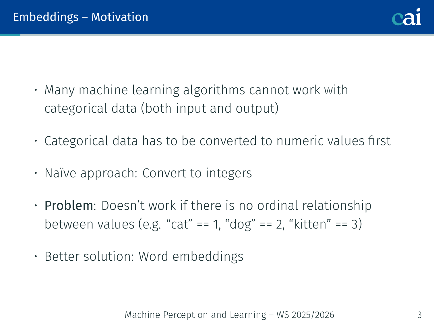
Embeddings are the secret sauce for handling categorical data in machine learning.

Many machine learning algorithms cannot work with categorical data directly — it must be converted to numeric values first.

Naïve approach: convert categories to integers (cat=1, dog=2, kitten=3).
Problem: this implies an ordinal relationship that doesn’t exist. There is no reason “kitten” should be numerically “between” cat and dog.

Better solution: Word embeddings — represent each word as a real-valued vector.

“You shall know a word by the company it keeps.” — Firth, 1957 (distributional hypothesis)

One-hot Encoding

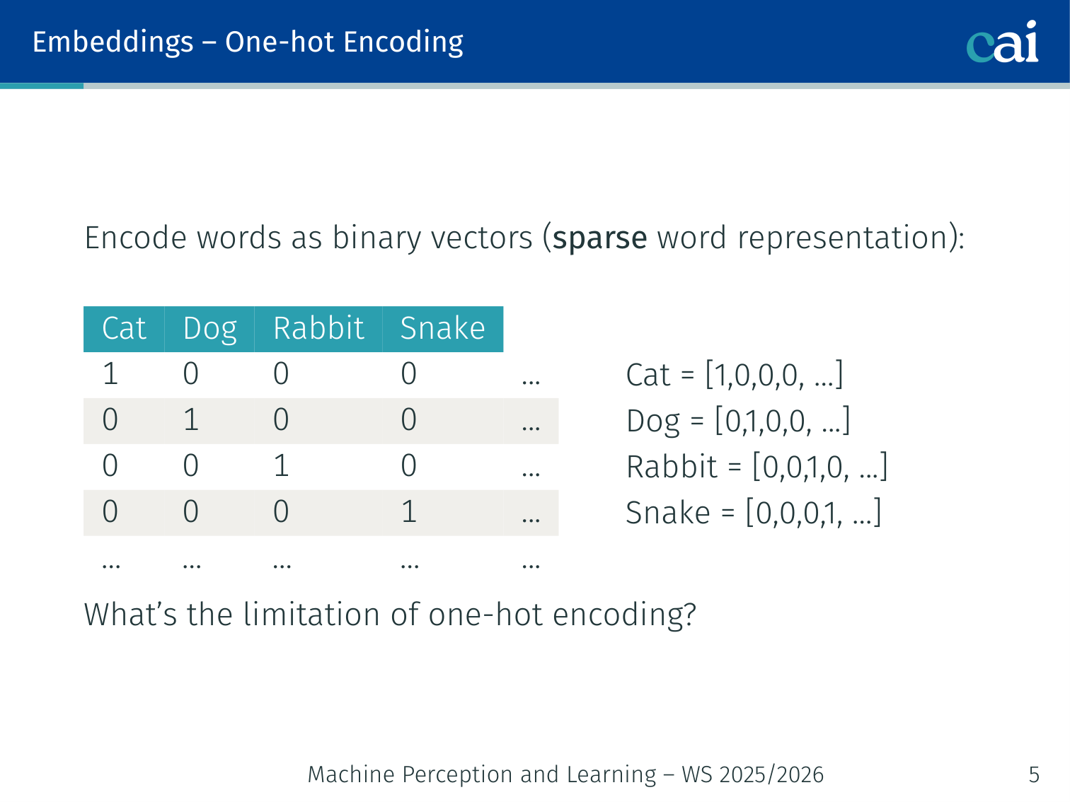
A quick look at how one-hot encoding represents words as sparse vectors.

Encode each word as a sparse binary vector of length $∣ V ∣$ (vocabulary size):

$cat = [1, 0, 0, 0, \dots]$ $dog = [0, 1, 0, 0, \dots]$ $rabbit = [0, 0, 1, 0, \dots]$

Limitation: all words are equally distant from each other — there is no notion of semantic similarity. “Cat” and “kitten” are just as far apart as “cat” and “airplane.”

Learned Embeddings

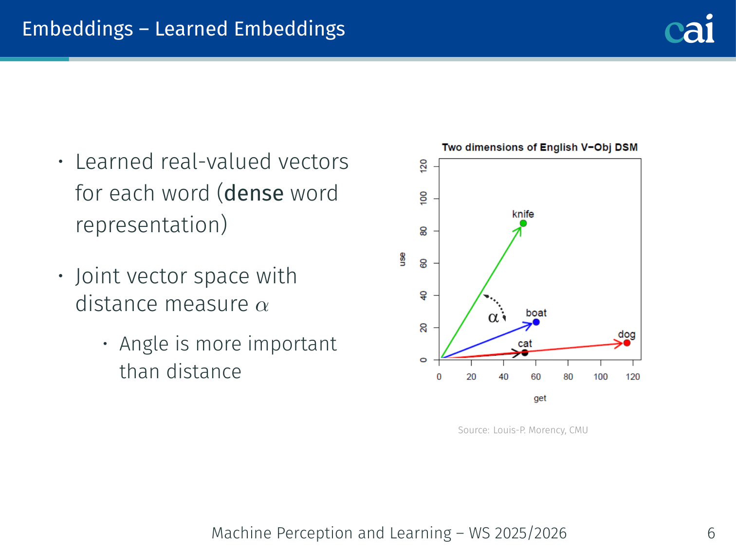
Learned embeddings map words into a space where similar meanings sit close together.

Instead of a sparse binary vector, map each word to a dense real-valued vector in a shared vector space. These vectors are learned from data.

Key properties:

Semantically similar words end up close in the embedding space
Angle (cosine similarity) is more informative than Euclidean distance
Algebraic relationships emerge:

$king - man + woman \approx queen$

This property reflects that the difference between gendered word pairs is captured consistently in the embedding space.

How to Learn Embeddings: CBOW and Skip-gram

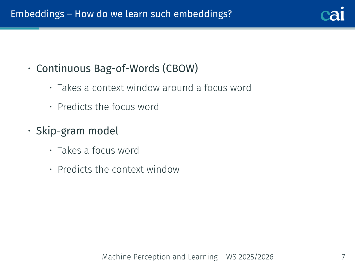
CBOW predicts a target word just by looking at the words surrounding it.

Skip-gram does the opposite: it uses one word to predict all the neighbors.

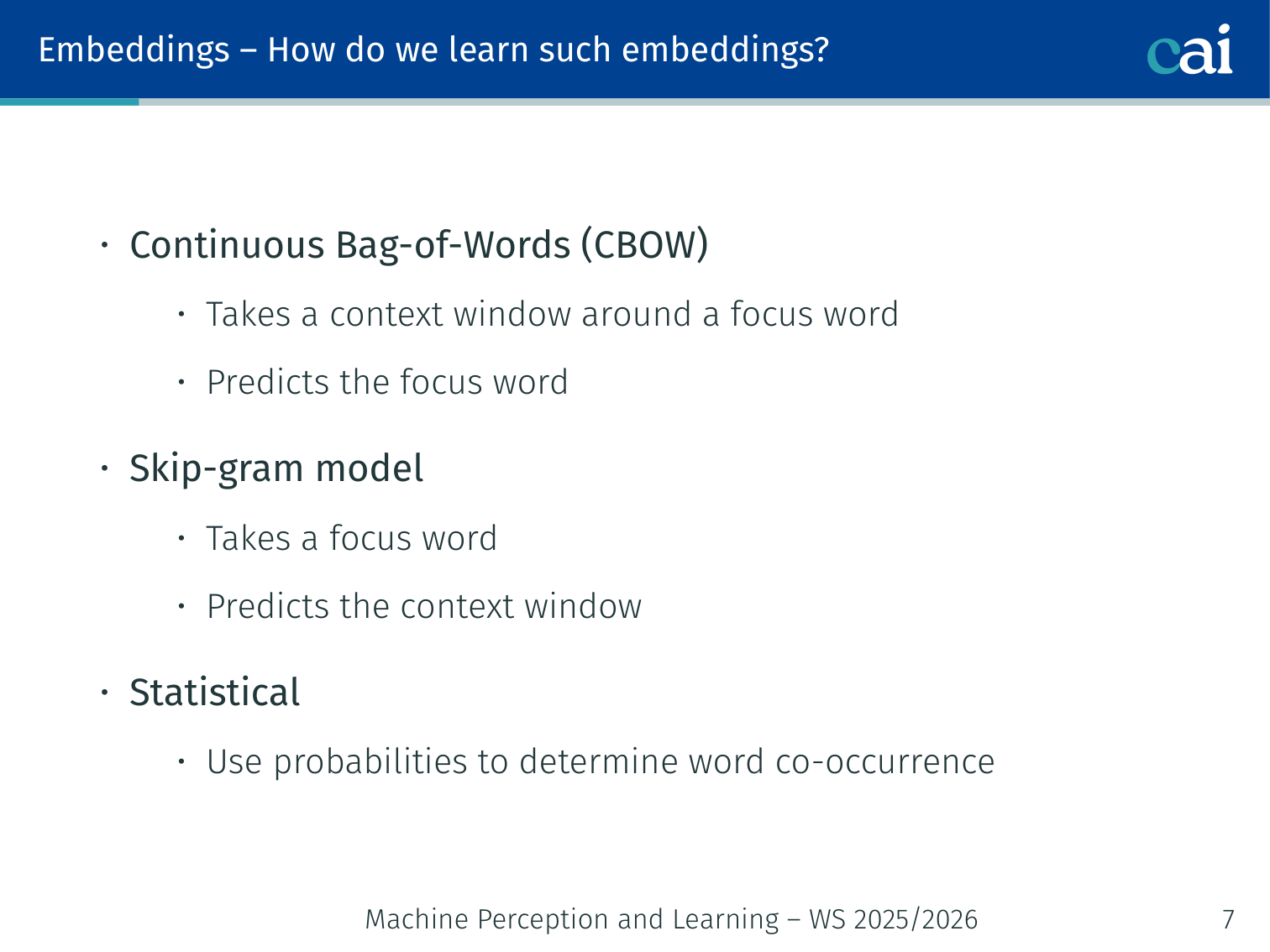
Three main approaches:

Continuous Bag-of-Words (CBOW): takes a context window around a focus word → predicts the focus word
Skip-gram: takes a focus word → predicts the context window
Statistical: uses co-occurrence probabilities across the whole corpus

CBOW is faster and works well for frequent words. Skip-gram better represents rare words.

CBOW:     [the, ___, sat, on]  →  "cat"
Skip-gram: "cat"               →  [the, sat, on, mat]

Word2Vec (Mikolov et al., 2013)

Word2Vec maps words into a space where relationships like "king - man + woman = queen" actually work.

Word2Vec is a family of shallow neural network models that learn word embeddings from a large corpus.

Trained on Google News dataset: 100 billion words
Uses a local context window for context
Can be trained as CBOW or Skip-gram

from gensim.models import Word2Vec
 
sentences = [["the", "cat", "sat", "on", "the", "mat"],
             ["the", "dog", "ran", "in", "the", "park"]]
 
model = Word2Vec(sentences, vector_size=100, window=5, min_count=1, sg=1)  # sg=1 → Skip-gram
 
# Word analogies
# king - man + woman ≈ queen
result = model.wv.most_similar(positive=["king", "woman"], negative=["man"], topn=1)
print(result)  # → [("queen", 0.87)]
 
# Semantic similarity
print(model.wv.similarity("cat", "dog"))    # high (both animals)
print(model.wv.similarity("cat", "table"))  # low

GloVe (Pennington et al., 2014)

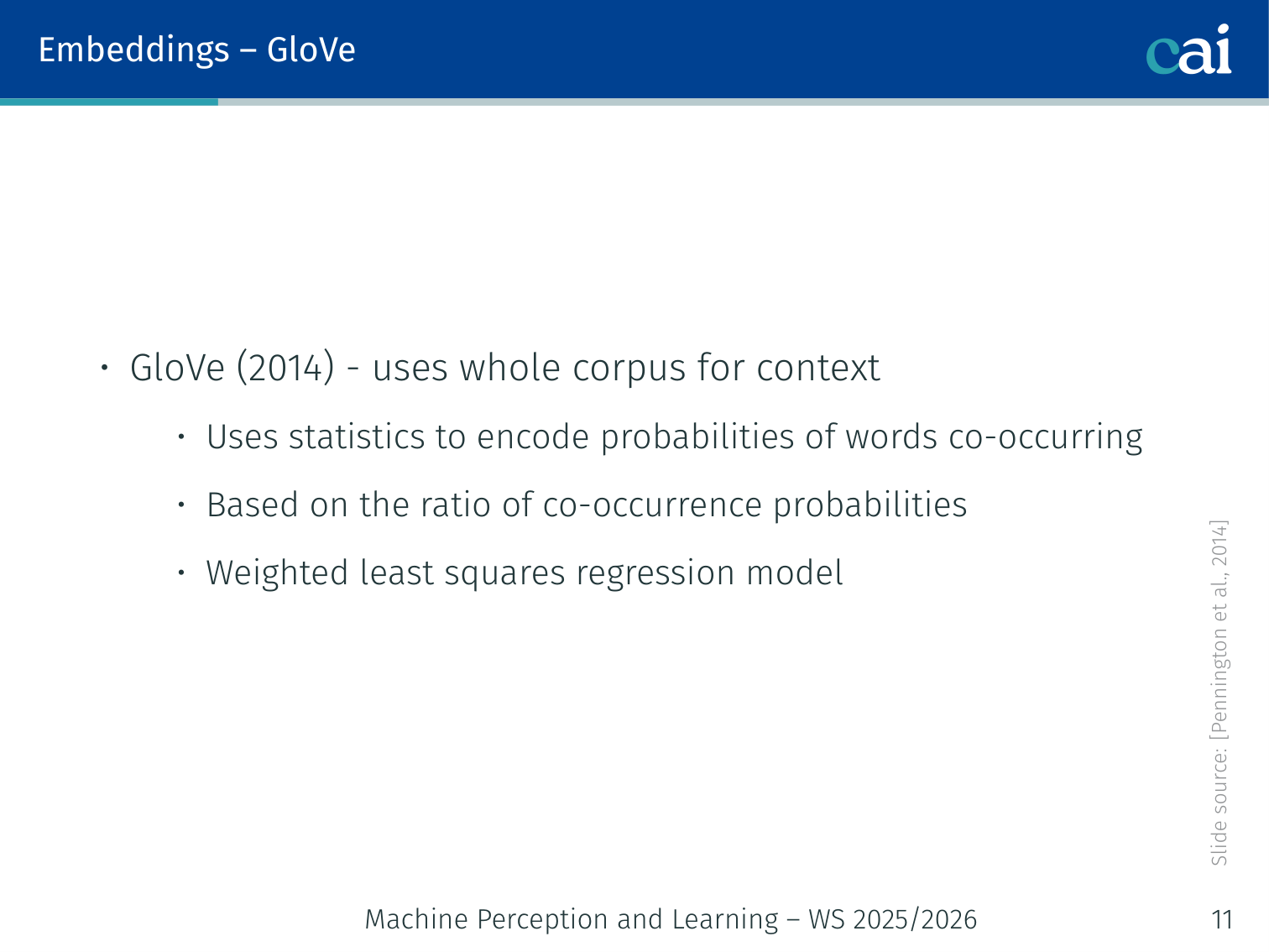
GloVe takes a global view, looking at how often words appear together across the whole dataset.

GloVe (Global Vectors) uses statistics from the entire corpus rather than a local window. It trains a weighted least-squares model on co-occurrence probabilities:

$J = \sum_{i, j} f (X_{ij}) (w_{i}^{⊤} \tilde{w}_{j} + b_{i} + \tilde{b}_{j} - lo g X_{ij})^{2}$

$X_{ij}$ : co-occurrence count of words $i$ and $j$
$f (X_{ij})$ : weighting function that downweights very frequent pairs
Captures both local and global structure
Often outperforms Word2Vec on word analogy benchmarks

GloVe example — gender analogy preserved across multiple pairs:

man → woman  same offset as:
king → queen
actor → actress
father → mother

Contextual vs. Non-Contextual Embeddings

Comparing classic embeddings with contextual ones—static vs. dynamic meanings.

The word "bank" can mean very different things; contextual embeddings finally help us tell them apart.

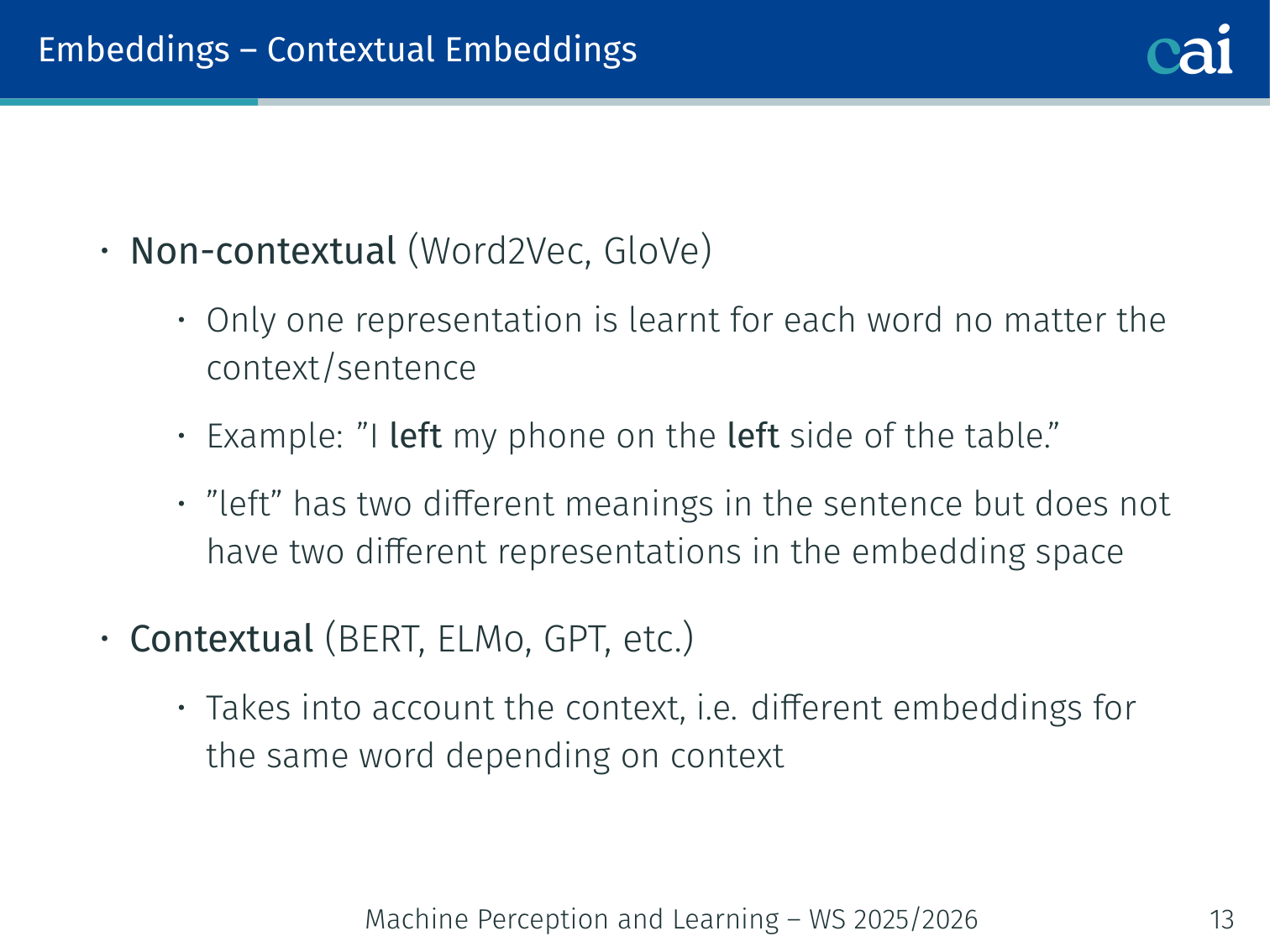
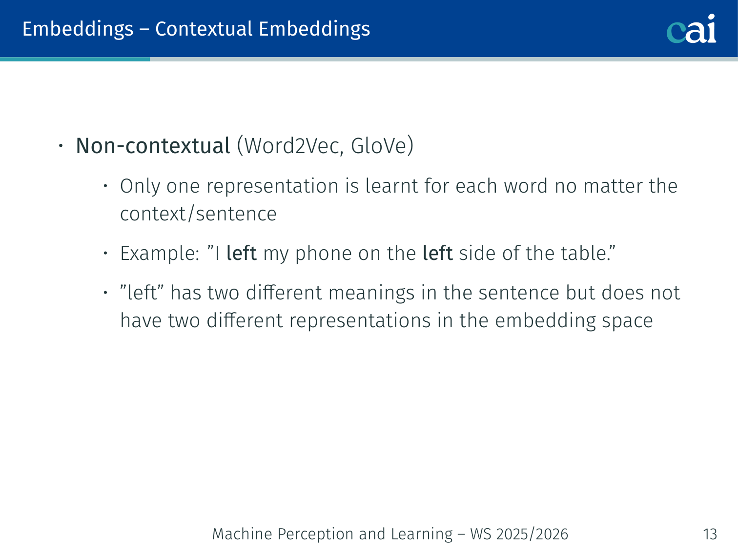
In Word2Vec and GloVe, each word has exactly one fixed vector regardless of context. But many words are polysemous:

“I left my phone on the left side of the table.”

The word “left” (past tense of leave) and “left” (spatial direction) are different meanings, but Word2Vec gives them the same embedding.

Contextual embeddings (ELMo, BERT, GPT) produce a different vector for each occurrence of a word, depending on its surrounding context.

Type	Examples	Representation
Non-contextual	Word2Vec, GloVe, FastText	One fixed vector per word type
Contextual	ELMo, BERT, GPT-2	Vector depends on sentence context

How Contextual Are Contextual Embeddings? (Ethayarajh, 2019)

As you go deeper into the Transformer, the embeddings get more and more specific to their context.

Ethayarajh (2019) compared BERT, ELMo, and GPT-2 using three new years: self-similarity, intra-sentence similarity, and Maximum Explainable Variance (MEV) — the proportion of variance in a word’s representations that can be explained by its first principal component.

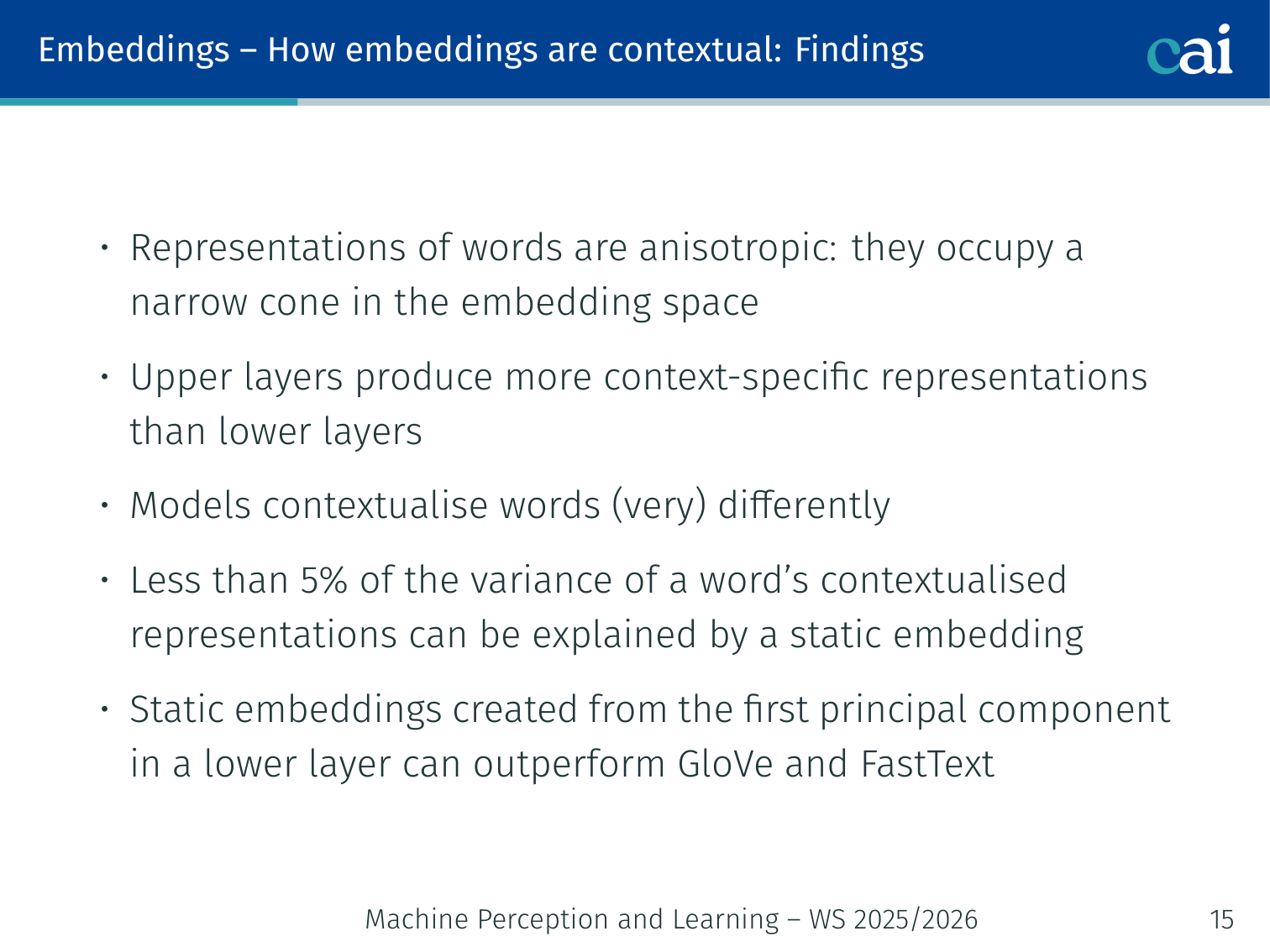
Findings:

Representations of words are anisotropic — they occupy a narrow cone in the embedding space (not uniformly distributed)
Upper layers produce more context-specific representations than lower layers
Models contextualise words very differently from one another
Less than 5% of the variance of a word’s contextualised representations can be explained by a static embedding
Static embeddings created from the first principal component of a lower layer can outperform GloVe and FastText

Attention Mechanisms

Motivation: RNN Weaknesses

RNNs struggle with long sequences because they process everything one step at a time.

The "bottleneck" happens when you try to squeeze a whole sentence into a single fixed-size vector.

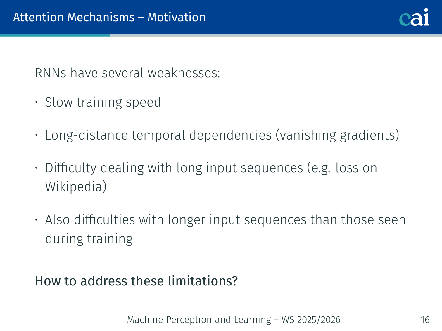
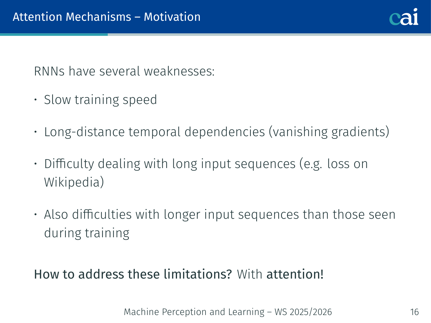
RNNs have several fundamental weaknesses that motivated the development of attention:

Slow training speed: computation is inherently sequential — step $t$ depends on step $t - 1$
Long-distance temporal dependencies: vanishing gradients prevent learning relationships between distant tokens
Difficulty with long input sequences: performance degrades on sequences longer than those seen during training
Fixed-size bottleneck: the encoder must compress an entire sequence into one vector

Solution: attention mechanisms!

Inspiration from Human Attention

Just like our eyes focus on specific parts of a scene, attention lets models focus on the most relevant data.

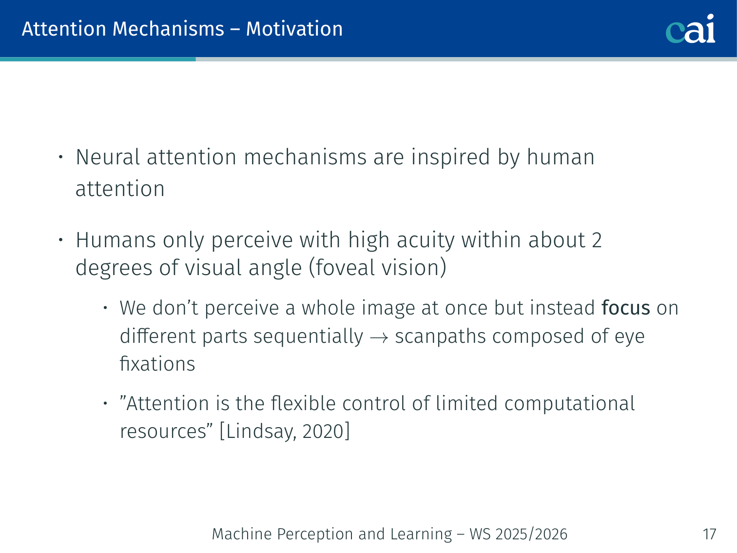
Neural attention is loosely inspired by human visual attention:

Humans perceive with high acuity only within ~2 degrees of visual angle (foveal vision)
We don’t perceive a whole image at once — we focus on different parts sequentially (scanpaths of eye fixations)
Neurons associated with the attended stimulus fire more synchronously

“Attention is the flexible control of limited computational resources.” — Lindsay, 2020

Attention in Machine Learning (Bahdanau et al., 2015)

Bahdanau attention lets the decoder "look back" at the encoder's states at every step.

You can actually see which words the model is focusing on as it translates from one language to another.

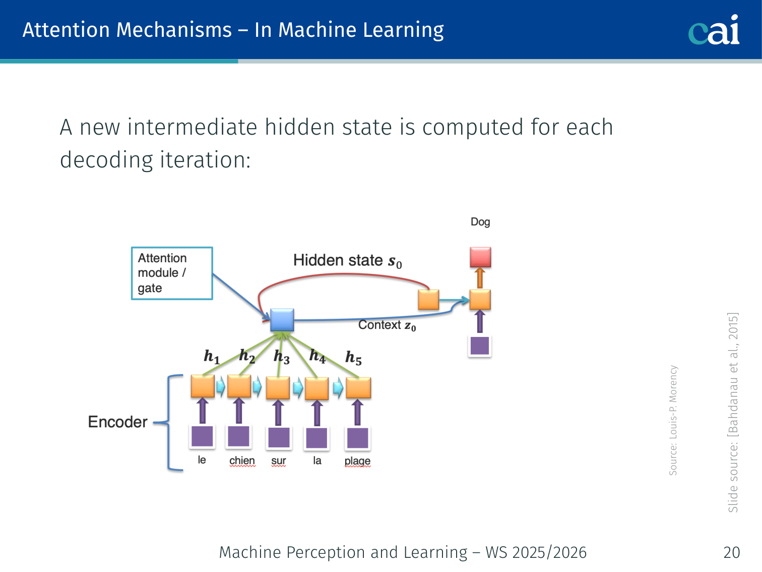
The original neural attention mechanism was introduced for machine translation (seq2seq). The problem: when decoding, you can only use the last encoder hidden state $h_{T}$ — a bottleneck for long sentences.

Before (standard seq2seq):

$p (y_{i} ∣ y_{1}, \dots, y_{i - 1}, x) = g (y_{i - 1}, s_{i}, z)$

where $z = h_{T}$ is just the final encoder state.

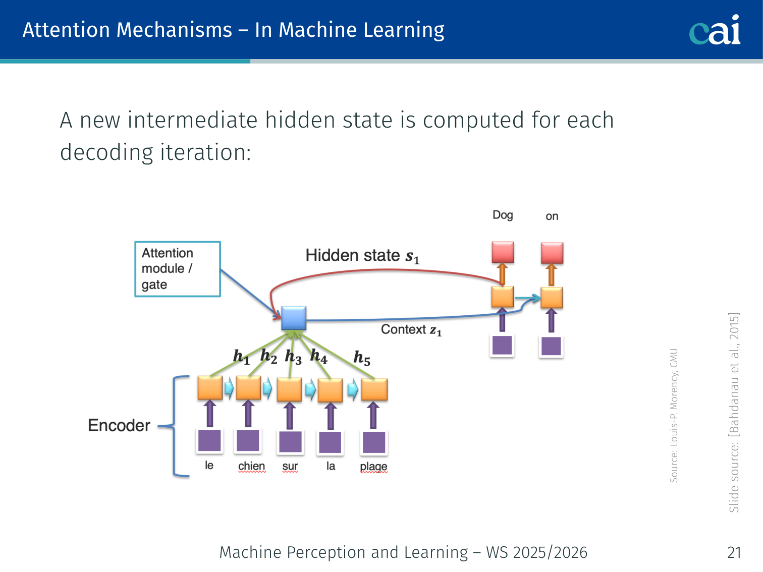
After (with attention):

$p (y_{i} ∣ y_{1}, \dots, y_{i - 1}, x) = g (y_{i - 1}, s_{i}, z_{i})$

A different context vector $z_{i}$ is computed at each decoding step:

$z_{i} = \sum_{j = 1}^{T_{x}} α_{ij} h_{j}$

This is a weighted sum over all encoder states $h_{j}$ , where $α_{ij}$ are the attention weights.

Computing the Attention Weights

This is the step-by-step process of how we calculate those all-important attention weights.

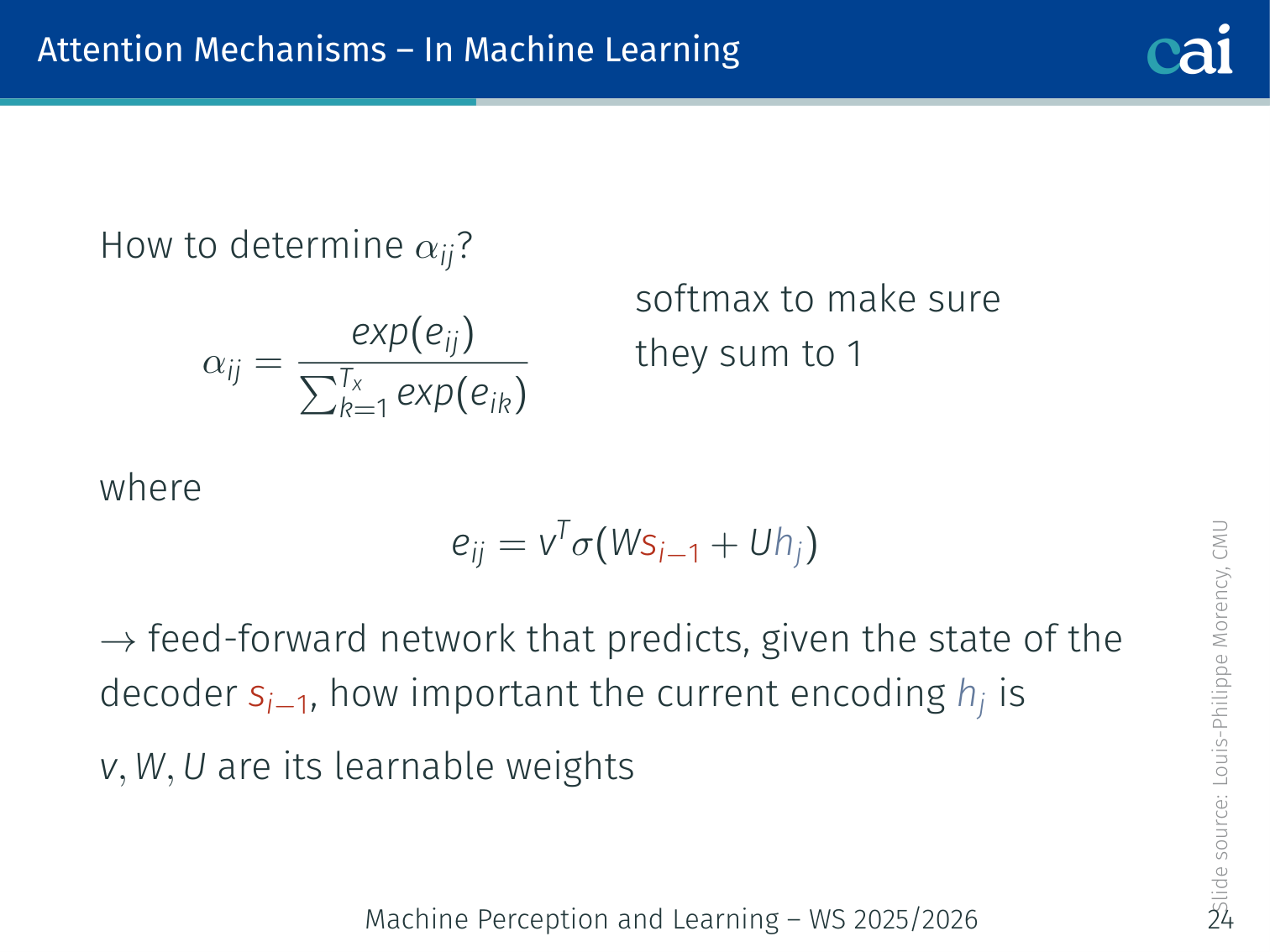
$α_{ij} = \frac{e x p ( e _{ij} )}{\sum _{k = 1}^{T_{x}} e x p ( e _{ik} )}$

(softmax to ensure they sum to 1)

where:

$e_{ij} = v^{⊤} σ (W s_{i - 1} + U h_{j})$

This is a small feed-forward network that scores, given the current decoder state $s_{i - 1}$ , how important each encoder output $h_{j}$ is. The parameters $v, W, U$ are learned jointly with the rest of the model.

Intuition: to generate the French word “zone”, the decoder can look back and put high attention on the English word “area” — directly, without having to “remember” it through a chain of hidden states.

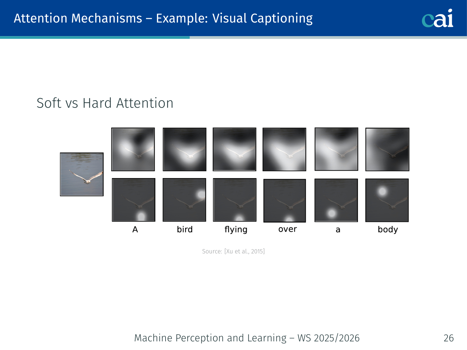
Soft vs. Hard Attention (Xu et al., 2015)

Soft attention is smooth and differentiable, while hard attention picks one spot and sticks to it.

	Soft Attention	Hard Attention
Method	Weighted average of all positions	Samples a single position
Differentiability	Differentiable (end-to-end)	Stochastic (requires REINFORCE)
Behaviour	”Looks” everywhere with varying focus	”Looks” at one area at a time
Human similarity	Less similar	More similar to human gaze

Example — visual captioning (Xu et al., 2015 — “Show, Attend and Tell”):
When generating the word “bird”, soft attention weights the entire image with a peak around the bird. Hard attention samples one patch — the bird’s location — and attends only there.

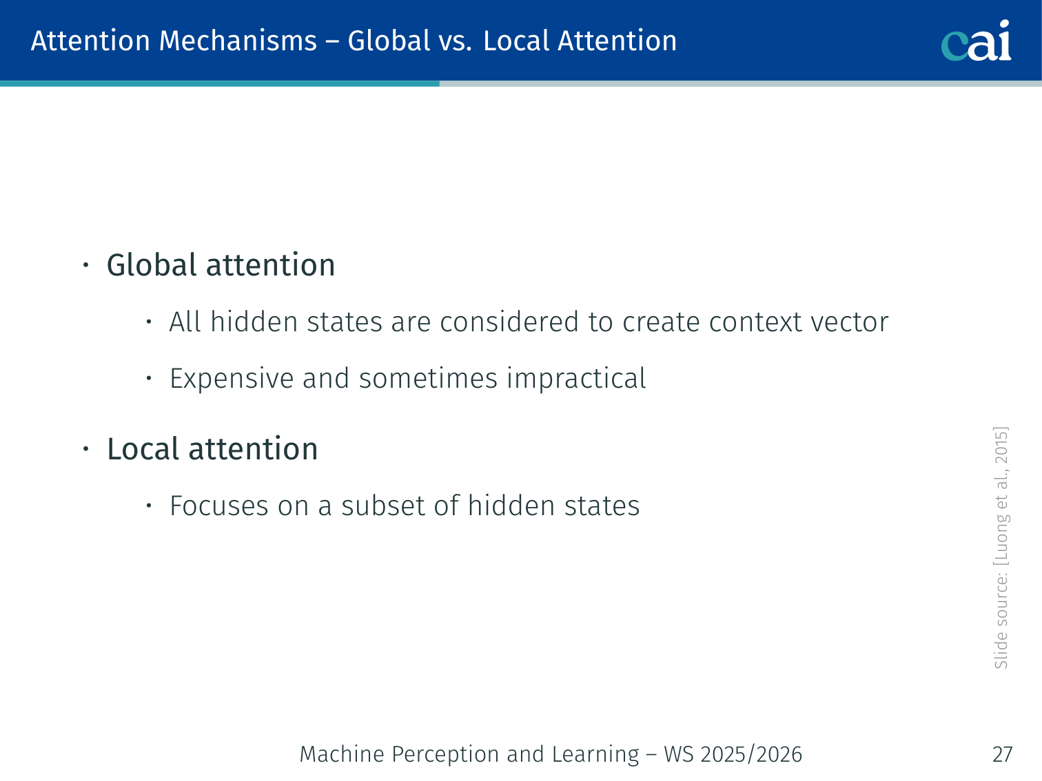
Global vs. Local Attention (Luong et al., 2015)

Global attention looks at everything, while local attention focuses on a small window of tokens.

	Global Attention	Local Attention
Scope	All encoder hidden states	Subset of hidden states
Cost	Expensive, $O (n)$ per step	Cheaper, $O (k)$ per step
Practical	OK for short sequences	Better for long sequences

In local attention, the model first predicts the “aligned position” $p_{t}$ for each decoder step, then attends only within a window $[p_{t} - D, p_{t} + D]$ .

Example — English-to-German translation (Luong et al., 2015):
For the output word “Wirtschaftszone”, global attention correctly puts weight on “economic” and “zone” in the source. Local attention achieves similar alignment but at a fraction of the cost for long documents.

Advantages of Attention

A quick recap of why attention is such a game-changer for neural networks.

Flexibility: handles variable-length inputs without a fixed-size bottleneck
Performance: significantly better on long sequences where RNNs degrade
Interpretability: the attention weights $α_{ij}$ are observable — you can visualise what the model is “looking at”

But: attention combined with RNNs is still slow due to sequential computation. The key insight of the Transformer: use attention only — remove recurrence entirely!

Attention Is All You Need

The landmark paper that introduced the world to the Transformer architecture.

Paper: Vaswani, Shazeer, Parmar, Uszkoreit, Jones, Gomez, Kaiser, Polosukhin. “Attention Is All You Need.” NeurIPS 2017. (202k+ citations)

Core idea:

Remove recurrence completely
Use only attention mechanisms
Stack multiple attention layers
Enables full parallelisation — massive speedup on GPUs

Architecture Overview

The Transformer is an encoder-decoder architecture:

Encoder: several identical encoder modules stacked (e.g., 6 in the original paper)
Decoder: several identical decoder modules stacked (e.g., 6)
No recurrence, no autoregressive hidden states

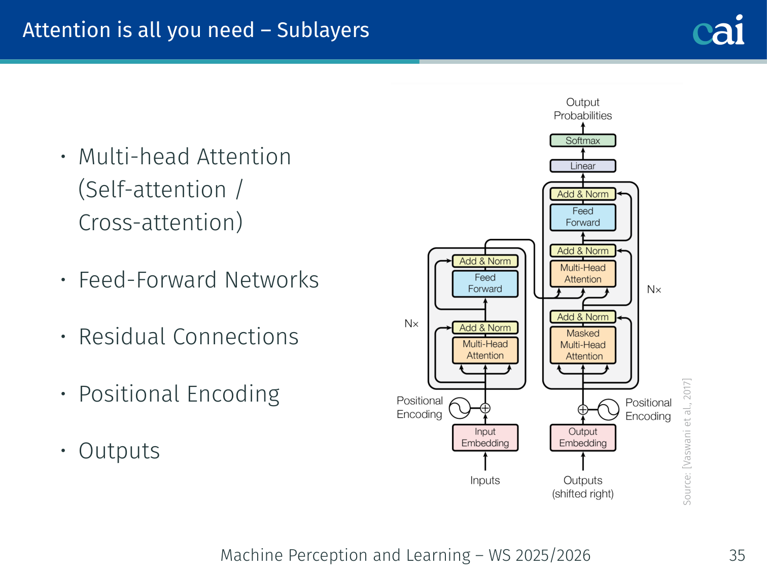
Sublayers in each block

The internal structure of a Transformer block—the building block of modern LLMs.

Multi-Head Attention (self-attention or cross-attention)
Feed-Forward Networks
Residual Connections + Layer Normalisation
Positional Encoding (added at input)

Self-Attention and Contextual Embeddings

Self-attention is what makes embeddings contextual. Each token produces three vectors from its embedding:

Query $q$ : “what information am I looking for?”
Key $k$ : “what information do I offer?”
Value $v$ : “what do I give if selected?”

For a sequence of $n$ tokens, each token attends to all $n$ tokens simultaneously (including itself). The attended-to information from all positions is blended into each position’s new representation — making it contextual.

Example: for the input “the cat sat on the mat”, the representation of “sat” after self-attention incorporates information from “cat” (the subject) and “mat” (the object), giving it a contextual understanding of the verb’s role.

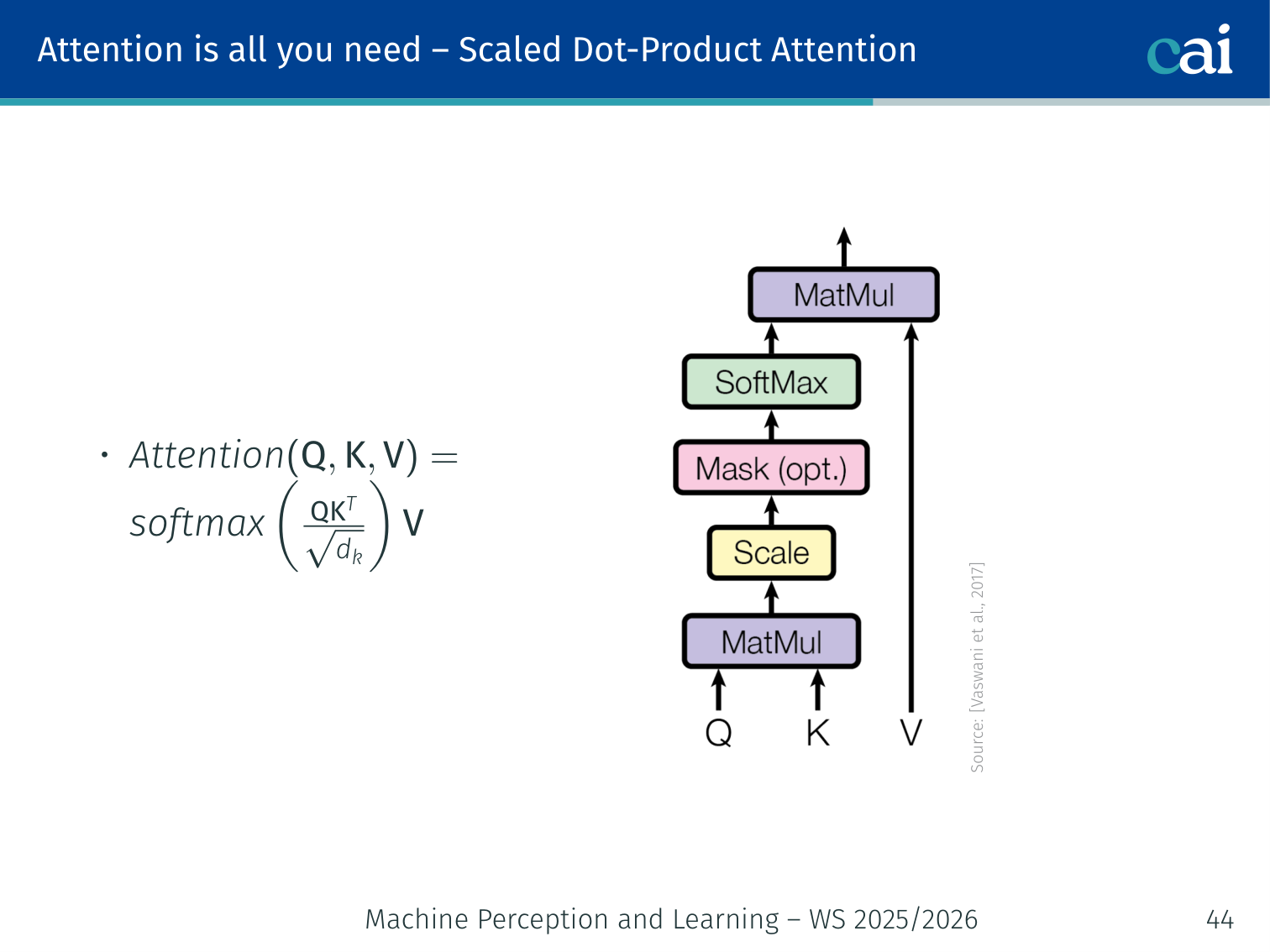
Scaled Dot-Product Attention

Scaled dot-product attention is the engine under the hood, using Queries, Keys, and Values.

$Attention (Q, K, V) = softmax (\frac{Q K ^{⊤}}{d _{k}}) V$

Step-by-step:

Compute dot products: $Q K^{⊤}$ — shape $(n \times n)$ , entry $(i, j)$ scores how relevant token $j$ is to token $i$
Scale by $\frac{1}{d _{k}}$ — prevents dot products from growing large in high dimensions and saturating softmax
Apply softmax — produces attention weights that sum to 1 per row
Weighted sum of values $V$ — produces the output

💡 Intuition: What the Attention Matrix Really Stores

The matrix

$A = softmax (\frac{Q K ^{⊤}}{d _{k}})$

is easiest to read row by row.

Row $i$ tells you: “when token $i$ updates itself, how much should it borrow from every token $j$ ?”
Entry $A_{ij}$ is a weight between 0 and 1.
Because each row sums to 1, the new representation of token $i$ is a weighted average of the value vectors.

So self-attention is not copying one token into another. It is building a context-aware mixture:

$output_{i} = \sum_{j} A_{ij} v_{j}$

This is why attention can express both sharp behaviors (“look almost entirely at one token”) and soft behaviors (“blend information from several related tokens”).

💡 Intuition: Self-Attention as a “Soft” Database Query

Think of self-attention like a database search, but instead of getting one exact result, you get a “blurry” mixture of several results.

Query ( $Q$ ): What I am looking for (e.g., “I am the word ‘it’, I need to know which noun I refer to”).
Key ( $K$ ): What I contain (e.g., “I am the word ‘apple’, I am a fruit/noun”).
Value ( $V$ ): What I actually contribute (e.g., the semantic meaning of “apple”).

When “it” (Query) looks at “apple” (Key), they match well. The attention mechanism then takes a large “sip” of the Value of “apple” and mixes it into the representation of “it”.

🧠 Deep Dive: Why the $1/ d_{k}$ scaling?

You might wonder why we don’t just use the dot product $Q K^{⊤}$ directly.

The Problem: As the dimension $d_{k}$ grows, the magnitude of the dot product grows too. If $q$ and $k$ are independent random variables with mean 0 and variance 1, then their dot product $q \cdot k = \sum_{i = 1}^{d_{k}} q_{i} k_{i}$ has mean 0 and variance $d_{k}$ .

For $d_{k} = 512$ , the values in $Q K^{⊤}$ can be very large. When you pass these large values into Softmax, the function becomes extremely “peaked” (one value near 1, others near 0).

The Consequence:

Vanishing Gradients: The derivative of softmax in the flat regions is nearly zero. If the attention is too peaked, the model stops learning because gradients can’t flow back.
Lack of Nuance: The model forced to pick only one token, losing the ability to blend context.

The Solution: By dividing by $d_{k}$ , we push the variance of the dot product back to 1, keeping the softmax in a “warm” region where gradients are healthy and the model can attend to multiple tokens.

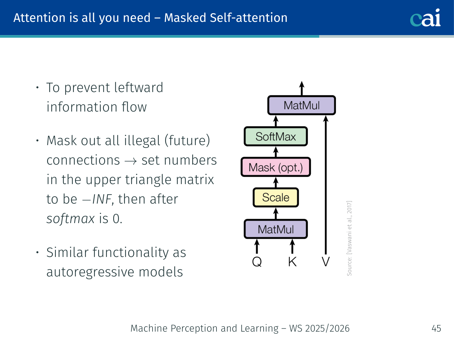
Masked Self-Attention

Causal masking ensures the model can't "cheat" by looking at future words during training.

In the decoder, when generating token $t$ , the model must not see future tokens $t + 1, t + 2, \dots$ — otherwise it would “cheat” by looking at the answer.

Fix: set entries in the upper triangle of the attention score matrix to $- \infty$ before softmax. After softmax, they become 0.

Scores (before masking):       After masking (upper tri → -∞):
[s11  s12  s13  s14]           [s11  -∞   -∞   -∞ ]
[s21  s22  s23  s24]    →      [s21  s22  -∞   -∞ ]
[s31  s32  s33  s34]           [s31  s32  s33  -∞ ]
[s41  s42  s43  s44]           [s41  s42  s43  s44]

After softmax, each row sums to 1, with zero weight on all future positions.

def causal_mask(seq_len):
    # Lower triangular: 1 = attend, 0 = mask
    return torch.tril(torch.ones(seq_len, seq_len)).unsqueeze(0)
 
mask = causal_mask(4)
# tensor([[[1, 0, 0, 0],
#           [1, 1, 0, 0],
#           [1, 1, 1, 0],
#           [1, 1, 1, 1]]])

Multi-Head Attention

Multi-head attention lets the model attend to different types of information in parallel.

One attention head learns one type of relationship. Multi-head attention runs $h$ attention operations in parallel, each in a lower-dimensional subspace:

$MultiHead (Q, K, V) = Concat (head_{1}, \dots, head_{h}) W^{O}$

$head_{i} = Attention (Q W_{i}^{Q}, K W_{i}^{K}, V W_{i}^{V})$

💡 Intuition: Multi-Head Attention as “Multiple Perspectives”

Imagine you are reading a mystery novel.

Head 1: Focuses on the names of the suspects (the “Who”).
Head 2: Focuses on the times and locations (the “When” and “Where”).
Head 3: Focuses on the tone of the dialogue (is the person lying?).

If you only had one “perspective”, you might miss a crucial detail. By using multiple heads, the Transformer can “see” the sentence in many different ways at the same time. One head might focus on grammar, while another focuses on the emotional meaning.

where:

$W_{i}^{Q} \in R^{d_{m o d e l} \times d_{q}}$
$W_{i}^{K} \in R^{d_{m o d e l} \times d_{k}}$
$W_{i}^{V} \in R^{d_{m o d e l} \times d_{v}}$

In the original paper: $d_{m o d e l} = 512$ , $h = 8$ , so $d_{k} = d_{v} = 64$ .

Why multi-head? Different heads can jointly attend to information from different representation subspaces at different positions. One head may track subject-verb agreement; another may track co-reference; another may track syntactic dependency.

Output: each head produces a $d_{v}$ -dimensional vector; these are concatenated and re-projected by $W^{O} \in R^{h \cdot d_{v} \times d_{m o d e l}}$ .

import torch
import torch.nn as nn
import math
 
class MultiHeadAttention(nn.Module):
    def __init__(self, d_model, h):
        super().__init__()
        assert d_model % h == 0
        self.d_k = d_model // h
        self.h = h
        self.W_q = nn.Linear(d_model, d_model)
        self.W_k = nn.Linear(d_model, d_model)
        self.W_v = nn.Linear(d_model, d_model)
        self.W_o = nn.Linear(d_model, d_model)
 
    def forward(self, Q, K, V, mask=None):
        B, T, D = Q.shape
        # Project and reshape to (B, h, T, d_k)
        q = self.W_q(Q).view(B, T, self.h, self.d_k).transpose(1, 2)
        k = self.W_k(K).view(B, -1, self.h, self.d_k).transpose(1, 2)
        v = self.W_v(V).view(B, -1, self.h, self.d_k).transpose(1, 2)
 
        scores = torch.matmul(q, k.transpose(-2, -1)) / math.sqrt(self.d_k)
        if mask is not None:
            scores = scores.masked_fill(mask == 0, float('-inf'))
        weights = torch.softmax(scores, dim=-1)
 
        out = torch.matmul(weights, v)                        # (B, h, T, d_k)
        out = out.transpose(1, 2).contiguous().view(B, T, D)  # (B, T, D)
        return self.W_o(out)

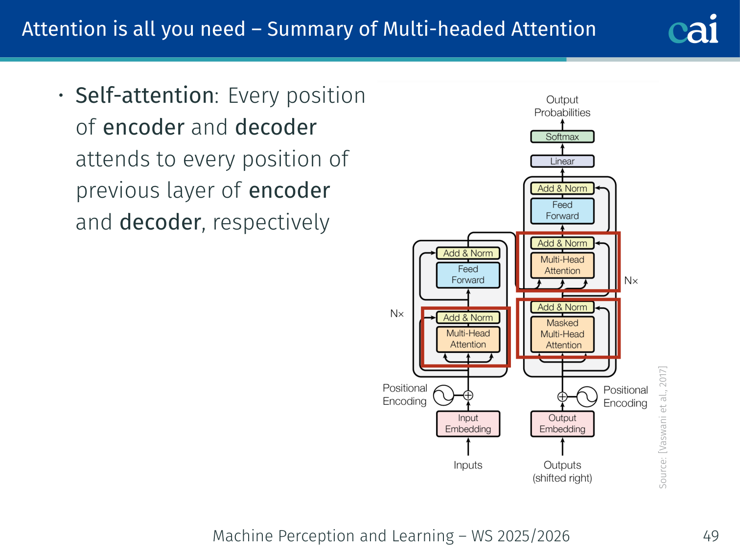
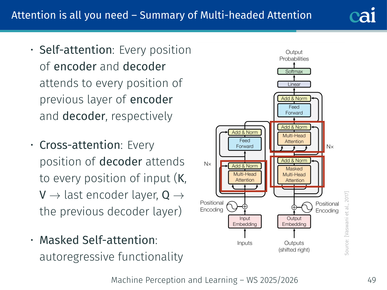
Summary of Multi-Head Attention Usage

Self-attention looks within the sequence, while cross-attention links the encoder and decoder.

A bird's-eye view of how different attention mechanisms are used throughout the model.

Context	Who attends to what
Self-attention (encoder)	Every encoder position attends to every other encoder position
Self-attention (decoder)	Every decoder position attends to all previous decoder positions (masked)
Cross-attention (decoder)	Every decoder position attends to every encoder position ( $K, V$ from encoder, $Q$ from decoder)

Feed-Forward Networks (FFN)

The feed-forward network adds some much-needed non-linearity after the attention layers.

The FFN is applied to every token separately, which makes it very efficient for parallel processing.

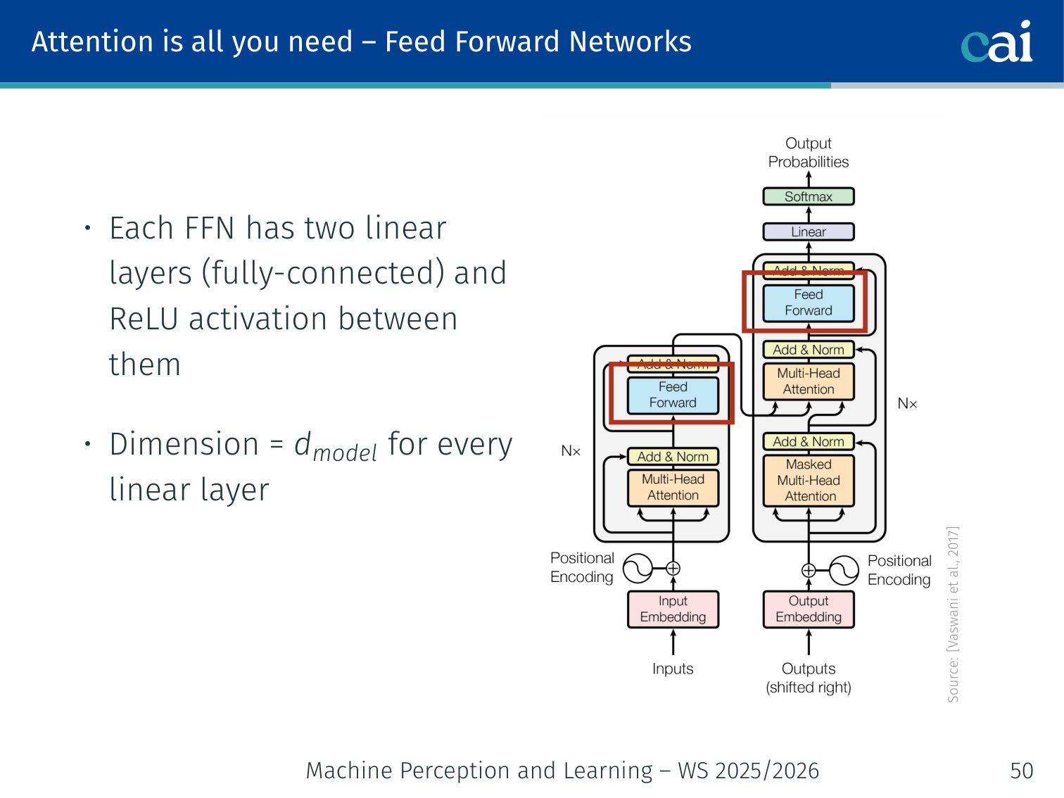
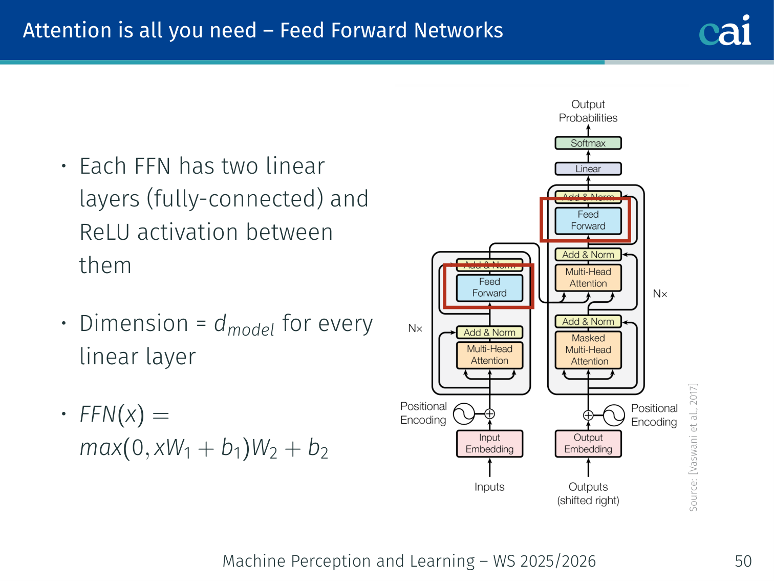
Each encoder/decoder block also contains a position-wise feed-forward network — a two-layer MLP applied independently to each position:

$FFN (x) = max (0, x W_{1} + b_{1}) W_{2} + b_{2}$

Two linear layers with a ReLU in between
Same $W_{1}, W_{2}$ are used at every position (but different from layer to layer)
In the original paper: $d_{m o d e l} = 512$ , inner dimension = $2048$ (4× expansion)

The FFN is where much of the model’s “knowledge” is stored — it can be seen as associative memory using the key-value structure of attention for routing, and FFN for retrieval.

💡 Intuition: Attention Lets Tokens Communicate, FFN Lets Them Think

One very useful mental model is:

Attention = communication between positions
FFN = computation performed inside each position

After attention, a token has gathered the context it needs from other tokens. The FFN then processes that enriched representation locally, without mixing it with neighboring positions again.

So each Transformer block has a two-step rhythm:

Look around with attention
Process what you learned with the FFN

This is why removing the FFN would make the model much weaker. Attention alone decides where information should flow, but the FFN helps transform that information into a better representation.

class FeedForward(nn.Module):
    def __init__(self, d_model, d_ff=2048):
        super().__init__()
        self.net = nn.Sequential(
            nn.Linear(d_model, d_ff),
            nn.ReLU(),
            nn.Linear(d_ff, d_model),
        )
 
    def forward(self, x):
        return self.net(x)  # Applied identically to each position

Residual Connections and Layer Normalisation

Residual connections and layer norm keep the training stable and the gradients flowing.

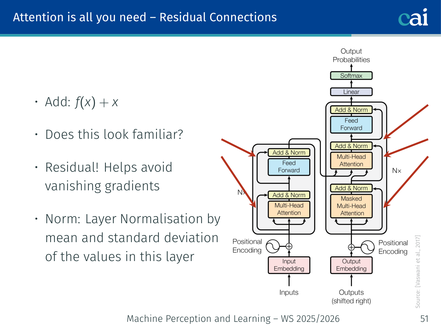
Each sublayer (attention or FFN) uses a residual connection:

$output = LayerNorm (x + sublayer (x))$

Residual connections (Add: $f (x) + x$ ) help avoid vanishing gradients — the same idea as ResNets (L03).

Layer Normalisation: normalizes by the mean and standard deviation of the activations within a single sample (across the feature dimension), not across the batch. This is essential because sequence lengths vary and batch statistics would be unreliable.

$LayerNorm (x) = γ \cdot \frac{x - μ}{σ + ϵ} + β$

where $μ$ and $σ$ are computed over the $d_{m o d e l}$ features for each token independently.

🧠 Deep Dive: Why Residuals and LayerNorm Matter So Much

Without these two ingredients, deep Transformers are much harder to optimize.

Residual connection says: “don’t destroy the old representation unless the sublayer has a good reason to change it.”
LayerNorm says: “keep the scale of activations under control so later layers see numerically stable inputs.”

Together they make each sublayer behave more like a correction to the current representation than a total rewrite of it. That is a big reason deep stacks remain trainable.

Another practical intuition:

attention can create very uneven activations depending on which tokens match strongly
FFNs can amplify some dimensions much more than others
LayerNorm re-centers and re-scales those outputs so the next block starts from a stable baseline

class TransformerBlock(nn.Module):
    def __init__(self, d_model, h, d_ff):
        super().__init__()
        self.attn = MultiHeadAttention(d_model, h)
        self.ff = FeedForward(d_model, d_ff)
        self.norm1 = nn.LayerNorm(d_model)
        self.norm2 = nn.LayerNorm(d_model)
 
    def forward(self, x, mask=None):
        x = self.norm1(x + self.attn(x, x, x, mask))  # Add & Norm
        x = self.norm2(x + self.ff(x))                # Add & Norm
        return x

Positional Encoding

Since Transformers don't have recurrence, we use these sine waves to tell the model where each word is.

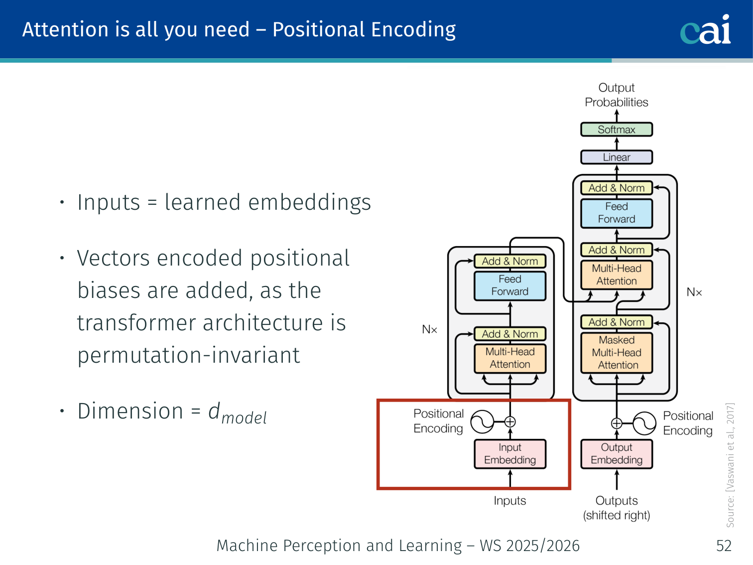
The Transformer architecture is permutation-invariant — self-attention treats the input as a set, not a sequence. To inject order information, a positional encoding is added to the input embeddings before the first layer.

The original paper uses sinusoidal encodings (no learned parameters):

$PE (p os, 2 i) = sin (\frac{p os}{1000 0 ^{2 i / d_{m o d e l}}})$

$PE (p os, 2 i + 1) = cos (\frac{p os}{1000 0 ^{2 i / d_{m o d e l}}})$

Each position $p os$ gets a unique vector of dimension $d_{m o d e l}$
Each dimension $i$ corresponds to a different frequency sinusoid
Relative positions can be expressed as linear functions of each other (useful for generalising to longer sequences)

Modern alternatives:

Learned positional embeddings: treat position as a token ID and learn an embedding (used in BERT, GPT-2)
RoPE (Rotary Position Embedding): rotates Q and K vectors by their position before dot-product — used in LLaMA, GPT-NeoX

💡 Intuition: Why Adding Position Vectors Is Enough

At first, it can feel strange that we just add a positional vector instead of doing something more elaborate.

The key idea is that the token embedding tells the model what the token is, while the positional encoding tells it where the token is. Adding them creates one combined vector that carries both pieces of information.

For example, the embedding for the word “bank” can mean the same thing in both of these sequences:

“the bank approved the loan”
“we sat by the bank of the river”

But once position and surrounding context are mixed in, attention can learn very different relationships for each occurrence. The original Transformer paper specifically chose sinusoidal encodings because fixed offsets can be represented linearly, which helps the model reason about relative position as well as absolute position.

import torch
import math
 
def sinusoidal_pe(max_len, d_model):
    pe = torch.zeros(max_len, d_model)
    pos = torch.arange(0, max_len).unsqueeze(1).float()
    div = torch.exp(torch.arange(0, d_model, 2).float() * (-math.log(10000) / d_model))
    pe[:, 0::2] = torch.sin(pos * div)
    pe[:, 1::2] = torch.cos(pos * div)
    return pe  # (max_len, d_model)

Outputs

At the decoder output, the model applies a learned linear transformation followed by softmax to produce a probability distribution over the vocabulary for the next token:

$P (next token) = softmax (h_{t} W_{vocab} + b)$

The embedding weight matrix (dimension $d_{m o d e l} \times ∣ V ∣$ ) is often shared with the output projection, multiplied by $d_{m o d e l}$ as a scaling factor. This weight tying reduces the number of parameters and is used in BERT, GPT, and most modern transformers.

Complexity Analysis

Operation	Complexity per Layer
Self-Attention	$O (n^{2} \cdot d)$ — quadratic in sequence length
FFN	$O (n \cdot d^{2})$ — linear in sequence length

The $O (n^{2})$ cost is the main scalability bottleneck for long sequences. For $n = 512$ (BERT) it is fine; for $n = 100 k$ it is not.

🧠 Deep Dive: FlashAttention (The Memory Trick)

If the math of attention is $O (n^{2})$ , how do modern models like Claude or GPT-4 handle 100,000+ words at once?

The secret isn’t a different formula; it’s FlashAttention.

The Problem: Standard attention is “Memory Bound.” The GPU spends 90% of its time just moving the giant $n \times n$ attention matrix back and forth between its slow memory (HBM) and its fast memory (SRAM).

The Solution: FlashAttention uses a technique called Tiling.

It breaks the giant matrix into small “tiles” that fit perfectly into the GPU’s fast SRAM.
It computes the attention for each tile and “stitches” them together without ever writing the full $n \times n$ matrix to slow memory.
Result: It is much faster and uses far less memory, even though the final answer is exactly the same!

BERT

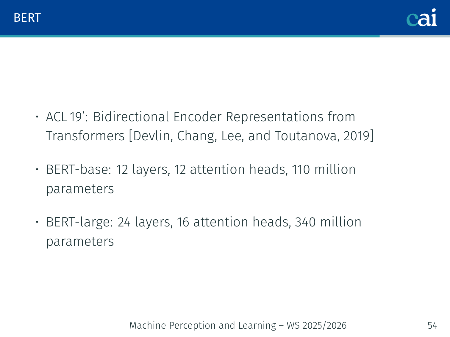
Paper: Devlin, Chang, Lee, Toutanova. “BERT: Pre-training of Deep Bidirectional Transformers for Language Understanding.” ACL 2019.

BERT is an encoder-only Transformer that produces contextual representations for every token, trained with self-supervised objectives on unlabeled text.

Architecture

BERT uses a stack of Transformer encoders to understand context from both directions at once.

Variant	Layers	Attention Heads	Parameters
BERT-base	12	12	110 million
BERT-large	24	16	340 million

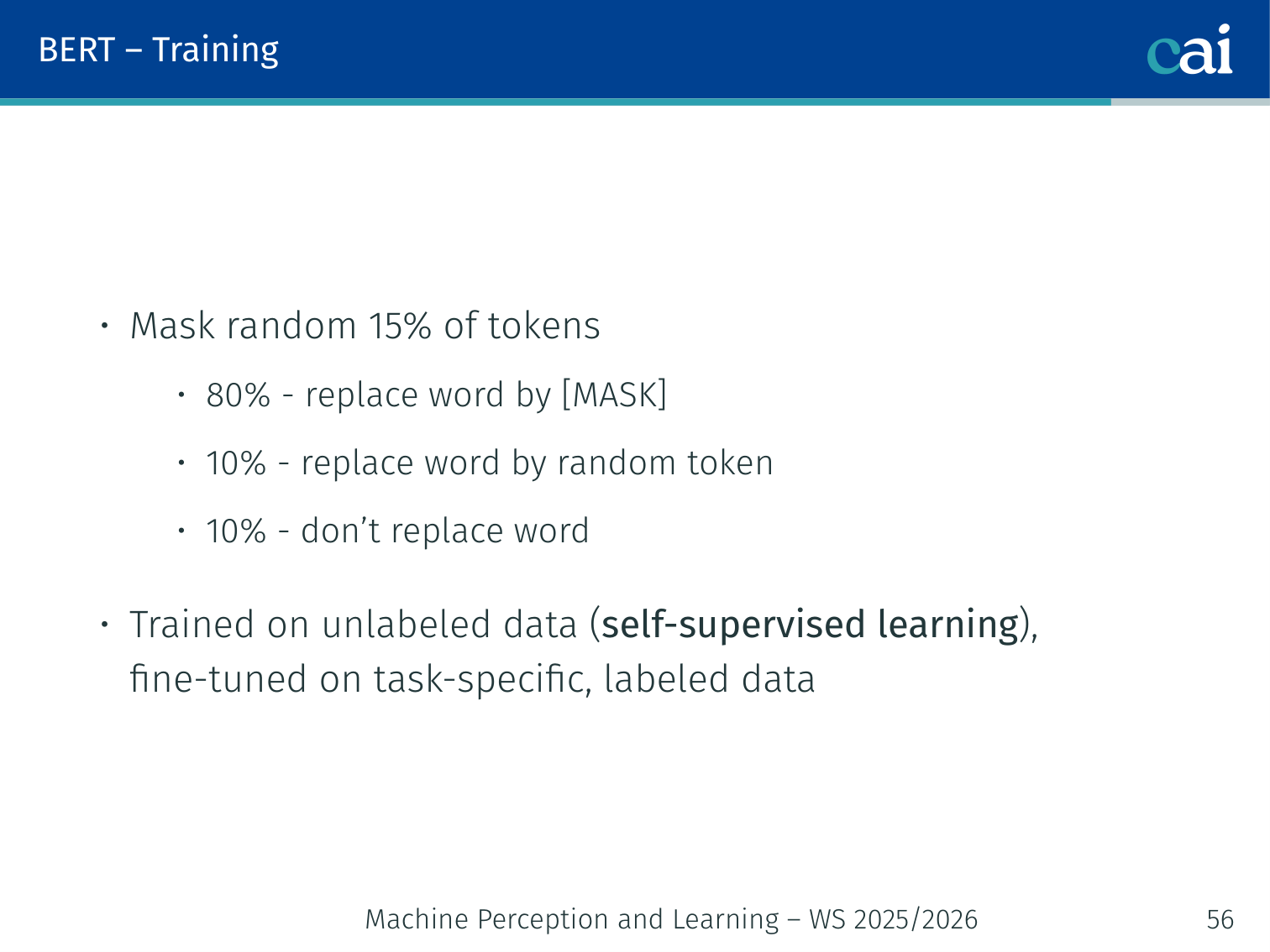
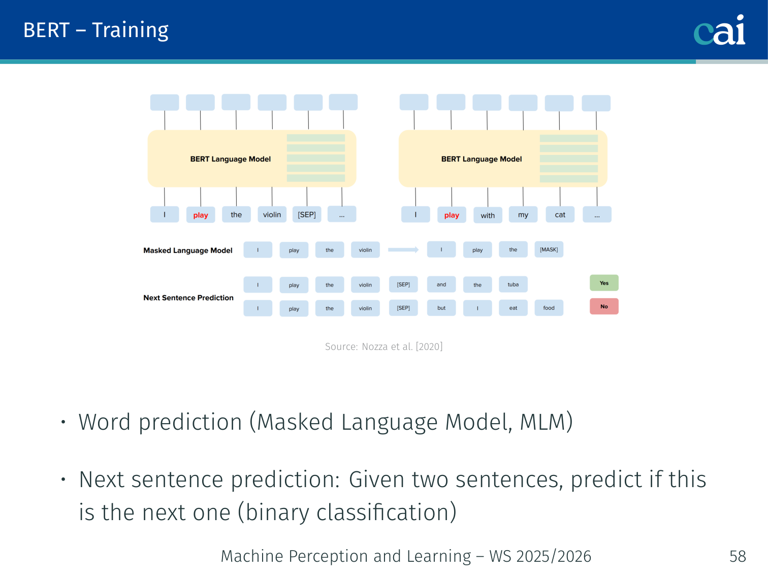
Pre-training: Two Objectives

1. Masked Language Model (MLM)

BERT learns by trying to fill in the blanks of sentences where some words are hidden.

Randomly mask 15% of input tokens, then predict the original tokens. Of the selected 15%:

80% — replace with [MASK]
10% — replace with a random token from the vocabulary
10% — keep the original token unchanged

This mixture prevents the model from only learning to predict [MASK] tokens.

Example:

Input:  "The [MASK] sat on the mat."
Target: predict "cat" at the [MASK] position

Input:  "The dog [MASK] on the mat."
Target: predict "sat" at the [MASK] position

Because [MASK] is seen during training but never at fine-tuning time, the 10% random and 10% unchanged tokens ensure the model must maintain a useful representation for every token — not just the masked ones.

2. Next Sentence Prediction (NSP)

The NSP task helps BERT understand the relationship between two different sentences.

Given two sentences A and B, predict whether B actually follows A in the corpus.

💡 Intuition: Why BERT Needed MLM Instead of Next-Token Prediction

The original BERT paper is built around one key idea: if you want a bidirectional encoder, ordinary next-token prediction is the wrong training objective.

In a causal LM, each token only sees the left context.
In a bidirectional encoder, each token can see both left and right context.

But if we let a bidirectional model predict every token while seeing the whole sentence, the answer would leak trivially. MLM avoids that by hiding some tokens, forcing the model to reconstruct them from the surrounding context.

That is why BERT’s pretraining recipe combines:

MLM to learn deep bidirectional token representations
NSP to learn relationships between paired spans

The BERT paper also emphasizes that the downstream architecture changes very little during fine-tuning, which is part of what made the approach so influential.

Input:  [CLS] The cat sat on the mat. [SEP] It was a warm afternoon. [SEP]
Label:  IsNext (True)

Input:  [CLS] The cat sat on the mat. [SEP] The stock market fell today. [SEP]
Label:  NotNext (False)

50% of training pairs are actual consecutive sentences; 50% are random pairings. The [CLS] (classification) token’s final representation is used to make the binary prediction.

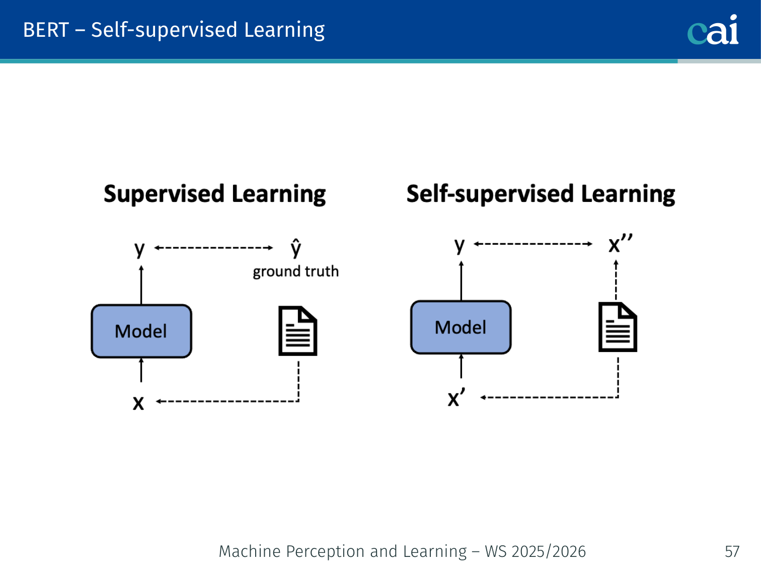
Self-supervised Learning

Self-supervised learning lets us train on massive amounts of raw text without needing manual labels.

BERT is trained with self-supervised learning — the labels (masked tokens, next sentence pairs) are derived automatically from unlabeled text, with no human annotation required. This allows training on massive datasets.

Training data:

BooksCorpus: 800 million words
English Wikipedia: 2,500 million words

Training time: 4 days on 64 TPU chips (BERT-large)

Fine-tuning on Downstream Tasks

After pre-training, BERT is fine-tuned on task-specific labeled data with minimal architectural changes:

Pre-training: unlabeled text → BERT weights
Fine-tuning:  labeled task data + BERT weights → task-specific model

Common fine-tuning tasks:

Task	How to use BERT	Example
Text classification	Use `[CLS]` token representation	Sentiment analysis
Named Entity Recognition	Use per-token representations	Label each word B-PER, I-PER, O, …
Question Answering	Predict start/end span in passage	SQuAD
Sentence pair tasks	Use `[CLS]` with two sentences	Natural language inference

from transformers import BertTokenizer, BertForSequenceClassification
import torch
 
tokenizer = BertTokenizer.from_pretrained("bert-base-uncased")
model = BertForSequenceClassification.from_pretrained("bert-base-uncased", num_labels=2)
 
# Sentiment classification
text = "This film was absolutely wonderful!"
inputs = tokenizer(text, return_tensors="pt", truncation=True, padding=True)
# inputs = {input_ids: ..., attention_mask: ..., token_type_ids: ...}
 
outputs = model(**inputs)
logits = outputs.logits          # (1, 2) — negative / positive
pred = logits.argmax(dim=-1)     # → 1 (positive)

Improved Variants

BERT set a new state-of-the-art across almost all NLP benchmarks when released and many variants followed:

RoBERTa (Liu et al., 2019): removes NSP objective, trains longer with larger batches, dynamic masking — significantly outperforms original BERT
ModernBERT (2024): a recent encoder-focused variant emphasizing efficiency and longer context

GPT — Decoder-only Transformers

GPT (“Generative Pre-trained Transformer”) takes the opposite design choice from BERT (Radford et al., 2018; Brown et al., 2020). Whereas BERT is encoder-only and bidirectional, GPT is decoder-only, autoregressive, and processes text strictly left-to-right.

BERT vs. GPT

Model	Architecture	Attention pattern	Pre-training objective	Typical use
BERT	Encoder-only	Bidirectional self-attention	MLM + NSP	Representation learning, classification, QA
GPT	Decoder-only	Causal (masked) self-attention	Next-token prediction	Text generation, prompting, in-context learning

Causal Self-Attention Only

GPT-style models use causal attention to predict the next word in a sequence, one by one.

A GPT block uses only masked self-attention. There is no encoder and, in the plain language-model setting, no cross-attention. Token $t$ may only attend to tokens at positions $\leq t$ .

Attention (Q, K, V) = softmax (\frac{Q K ^{⊤} + M}{d _{k}}) V

where the causal mask $M_{ij} = - \infty$ for $j > i$ and $0$ otherwise.

This mask prevents the model from “looking into the future” during training.

Pre-training Objective: Next-Token Prediction

GPT is trained as a standard language model:

p (x_{1}, \dots, x_{T}) = t = 1 \prod T p (x_{t} ∣ x_{< t})

so the loss is the negative log-likelihood of the next token:

L_{LM} = - t = 1 \sum T lo g p_{θ} (x_{t} ∣ x_{< t})

At every step, the model answers the same question: given the prefix so far, what token should come next?

Example: Prompt: The capital of France is

Target next token: Paris

Scaling: GPT-1 → GPT-2 → GPT-3

A major result of the GPT line is that simply scaling parameters and data leads to qualitatively new behaviour.

Model	Parameters	Training data	Key outcome
GPT-1	117M	BooksCorpus	Generative pre-training improves many NLP tasks after fine-tuning
GPT-2	1.5B	WebText	Stronger long-form generation; zero-shot behaviour starts to emerge
GPT-3	175B	Web-scale corpus (~300B tokens from Common Crawl, books, Wikipedia, etc.)	Clear few-shot prompting and in-context learning

As scale increases, GPT models become better at zero-shot, one-shot, and few-shot generalisation, even though the core decoder-only architecture stays the same (Brown et al., 2020).

Fine-tuning vs. Prompting

There are two common ways to adapt GPT models:

Strategy	How it works	Strength
Fine-tuning	Update model weights on task-specific labeled data	Best when you want a specialised model for one task
Prompting / in-context learning	Keep weights fixed and describe the task in the prompt, optionally with examples	No gradient updates needed; flexible across many tasks

Example:
Translate English to German.
 
dog -> Hund
cat -> Katze
house ->
The model infers the task from the prompt itself. This is in-context learning: the context changes the behaviour without changing the weights.

In short: BERT is mainly a bidirectional encoder for representation learning, while GPT is mainly a decoder-only model for autoregressive generation and prompting.

PyTorch Implementation: Transformer

The Transformer architecture completely replaces recurrence with Multi-Head Attention. Below is a simplified implementation using PyTorch’s built-in nn.Transformer module.

import torch
import torch.nn as nn
 
class TransformerModel(nn.Module):
    def __init__(self, src_vocab_size, tgt_vocab_size, d_model=512, nhead=8, num_layers=6):
        super().__init__()
        # 1. Embeddings: Convert discrete word IDs into dense vectors
        self.embedding_src = nn.Embedding(src_vocab_size, d_model)
        self.embedding_tgt = nn.Embedding(tgt_vocab_size, d_model)
 
        # 2. The Core Transformer: Handles both Encoder and Decoder logic
        # d_model: number of features in input vectors
        # nhead: number of parallel attention heads
        # num_layers: number of sub-layers in both encoder and decoder
        self.transformer = nn.Transformer(d_model, nhead, num_layers, num_layers)
 
        # 3. Final Linear Layer: Projects model output back to vocabulary size
        self.fc_out = nn.Linear(d_model, tgt_vocab_size)
 
    def forward(self, src, tgt):
        """
        Args:
            src: Source sequence indices, shape (S, N)
            tgt: Target sequence indices, shape (T, N)
            (S = Source length, T = Target length, N = Batch size)
        """
        # Embed the source and target tokens
        src_emb = self.embedding_src(src)
        tgt_emb = self.embedding_tgt(tgt)
 
        # PyTorch Transformer expects input shape: (Seq_Len, Batch, Embed_Dim)
        # It performs self-attention on src, self-attention on tgt,
        # and cross-attention between them automatically.
        out = self.transformer(src_emb, tgt_emb)
 
        # Project the resulting features to get logits for each vocabulary word
        return self.fc_out(out)

Key Transformer Concepts:

nn.Transformer: A black-box implementation of the entire Vaswani et al. (2017) architecture. It is highly optimized for performance.
Permutation Invariance: Notice that without “Positional Encodings” (omitted here for simplicity), the Transformer doesn’t know the order of words. In practice, you must add sinusoidal or learned vectors to the embeddings.
Parallelism: Unlike RNNs, the entire source sequence src is processed in one step, making Transformers much faster to train on modern hardware.

Summary

From the lecture’s closing slide:

Contextual embeddings (e.g., BERT) are better representations than non-contextual embeddings (e.g., Word2Vec)
Attention mechanism types:
- Soft vs. hard attention
- Local vs. global attention
- Self- vs. cross-attention
Transformer architecture uses only attention — no recurrence — enabling full parallelisation
BERT and its variants are the current SOTA for encoder representations
Training transformers takes a lot of training data, GPU memory, and time — a significant disadvantage compared to RNNs for small datasets

Real-World Application: The semantic understanding of Transformers is the core engine behind SlideLink, a tool I built to contextually align lecture notes with PDF slides.

Component	Key Point
One-hot encoding	Sparse, no similarity information
Word2Vec / GloVe	Dense, non-contextual, algebraic properties
Contextual embeddings	Different vector per context; upper layers more specific
Self-attention	Every token attends to every other — $O (n^{2})$
Scaled dot-product	$softmax (Q K^{⊤} / d_{k}) V$
Masked self-attention	Causal masking for autoregressive generation
Multi-head attention	$h$ parallel heads, different subspaces
Positional encoding	Sinusoidal or learned; added to embeddings
FFN	Per-position 2-layer MLP with ReLU
Residual + LayerNorm	Add & Norm — avoids vanishing gradients
BERT	Encoder-only, MLM + NSP, 110M–340M params
GPT	Decoder-only, causal self-attention, next-token prediction, strong zero-/few-shot prompting

References

Ba, Mnih, Kavukcuoglu (2014) — Multiple object recognition with visual attention. arXiv:1412.7755.
Bahdanau, Cho, Bengio (2015) — Neural machine translation by jointly learning to align and translate. ICLR.
Brown et al. (2020) — Language models are few-shot learners. NeurIPS.
Devlin, Chang, Lee, Toutanova (2019) — BERT: Pre-training of deep bidirectional transformers for language understanding. arXiv:1810.04805.
Ethayarajh (2019) — How contextual are contextualized word representations? arXiv:1909.00512.
Firth (1957) — Studies in linguistic analysis. Blackwell, Oxford.
Lindsay (2020) — Attention in psychology, neuroscience, and machine learning. Frontiers in Computational Neuroscience, 14:29.
Luong, Pham, Manning (2015) — Effective approaches to attention-based neural machine translation. arXiv:1508.04025.
Mikolov et al. (2013a) — Efficient estimation of word representations in vector space. arXiv:1301.3781.
Mikolov et al. (2013b) — Exploiting similarities among languages for machine translation. arXiv:1309.4168.
Mnih, Heess, Graves et al. (2014) — Recurrent models of visual attention. NeurIPS, pp. 2204–2212.
Nozza, Bianchi, Hovy (2020) — What the [MASK]? Making sense of language-specific BERT models. arXiv:2003.02912.
Pennington, Socher, Manning (2014) — GloVe: Global vectors for word representation. EMNLP, pp. 1532–1543.
Radford, Narasimhan, Salimans, Sutskever (2018) — Improving language understanding by generative pre-training. OpenAI technical report.
Radford et al. (2019) — Language models are unsupervised multitask learners. OpenAI technical report.
Vaswani et al. (2017) — Attention is all you need. NeurIPS, pp. 5998–6008.
Xu et al. (2015) — Show, attend and tell: Neural image caption generation with visual attention. ICML, pp. 2048–2057.

Applied Exam Focus

Self-Attention: Complexity is $O (N^{2})$ with respect to sequence length $N$ . This is the primary scaling bottleneck.
Multi-Head Attention: Allows the model to attend to different parts of the sequence simultaneously (e.g., one head for syntax, another for semantics).
Positional Encoding: Crucial because Transformers have no inherent sense of order (unlike RNNs). Without it, the model treats the input as a “bag of words.”

Previous: L04 — RNNs | Back to MPL Index | Next: (y-06) ViT | (y) Return to Notes | (y) Return to Home

Yusuf's Thoughts

Explorer