L06 — Vision Transformer (ViT)

Previous: L05 — Transformers | Back to MPL Index | Next: (y-07) Multimodal

This lecture covers:

Vision Transformer (ViT)
Object Detection with ViTs (DETR)
Self-supervised Vision Transformers (DINO)

Mental Model First

ViT treats an image as a sequence of patches, then applies the Transformer machinery from language.
CNNs bake in locality and translation bias; ViTs are more flexible but must learn more structure from data.
DETR shows that detection can be framed as set prediction, and DINO shows that strong visual representations can emerge even without labels.
If one question guides this lecture, let it be: what changes when we stop treating vision as a grid of convolutions and start treating it as a sequence problem?

Vision Transformer (ViT)

Limitations of CNNs

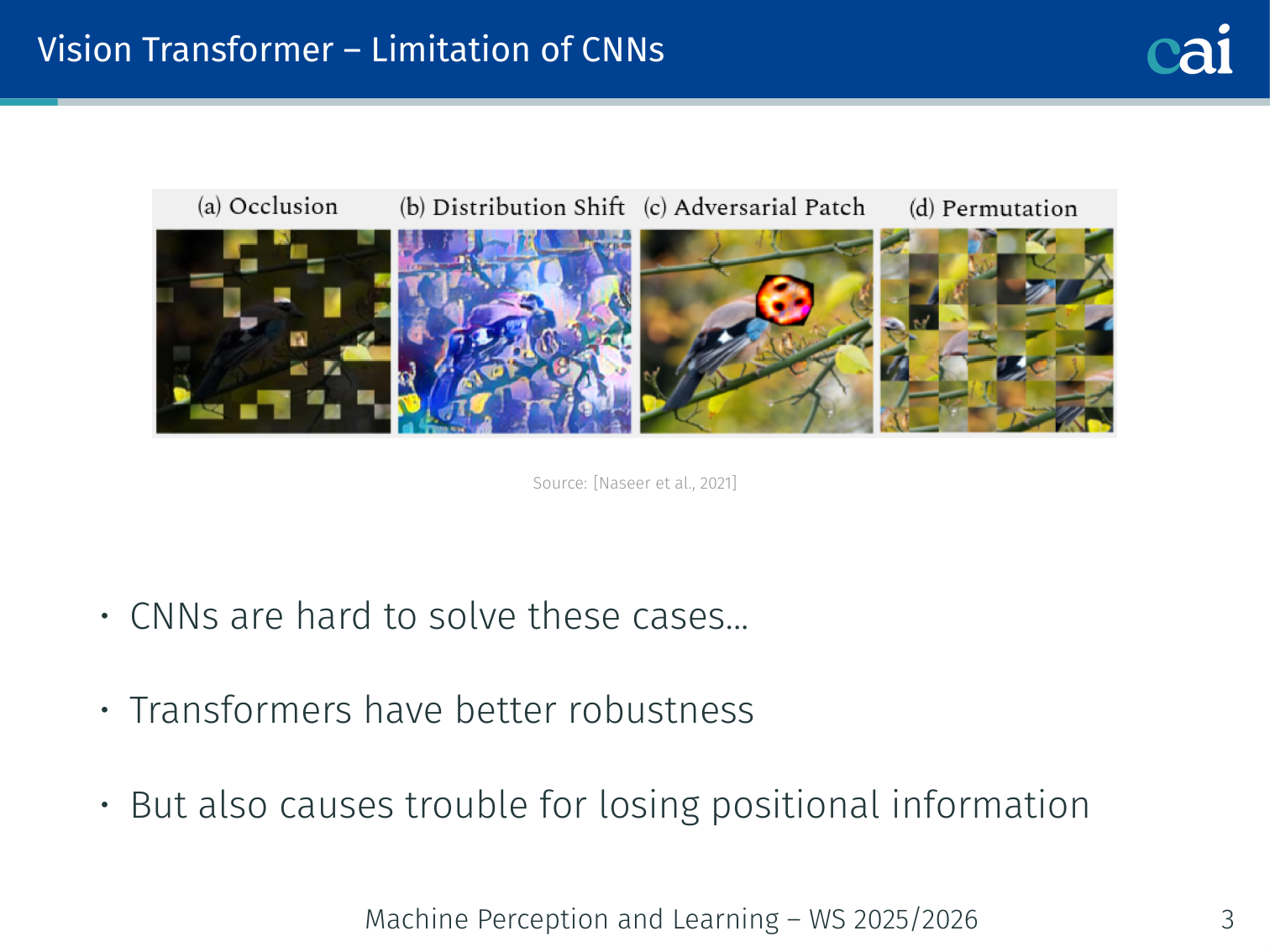
CNNs can be surprisingly fragile when it comes to changes in texture or distribution.

CNNs have several weaknesses that motivated looking at Transformer alternatives (Naseer et al., 2021):

CNNs are brittle to certain distribution shifts (adversarial texture changes, style transfer) that humans handle easily
Transformers show better robustness to such perturbations — because they are not constrained to local receptive fields
However, Transformers also cause trouble by losing positional information unless position is explicitly encoded

Replacing CNNs with Self-Attention (Ramachandran et al., 2019)

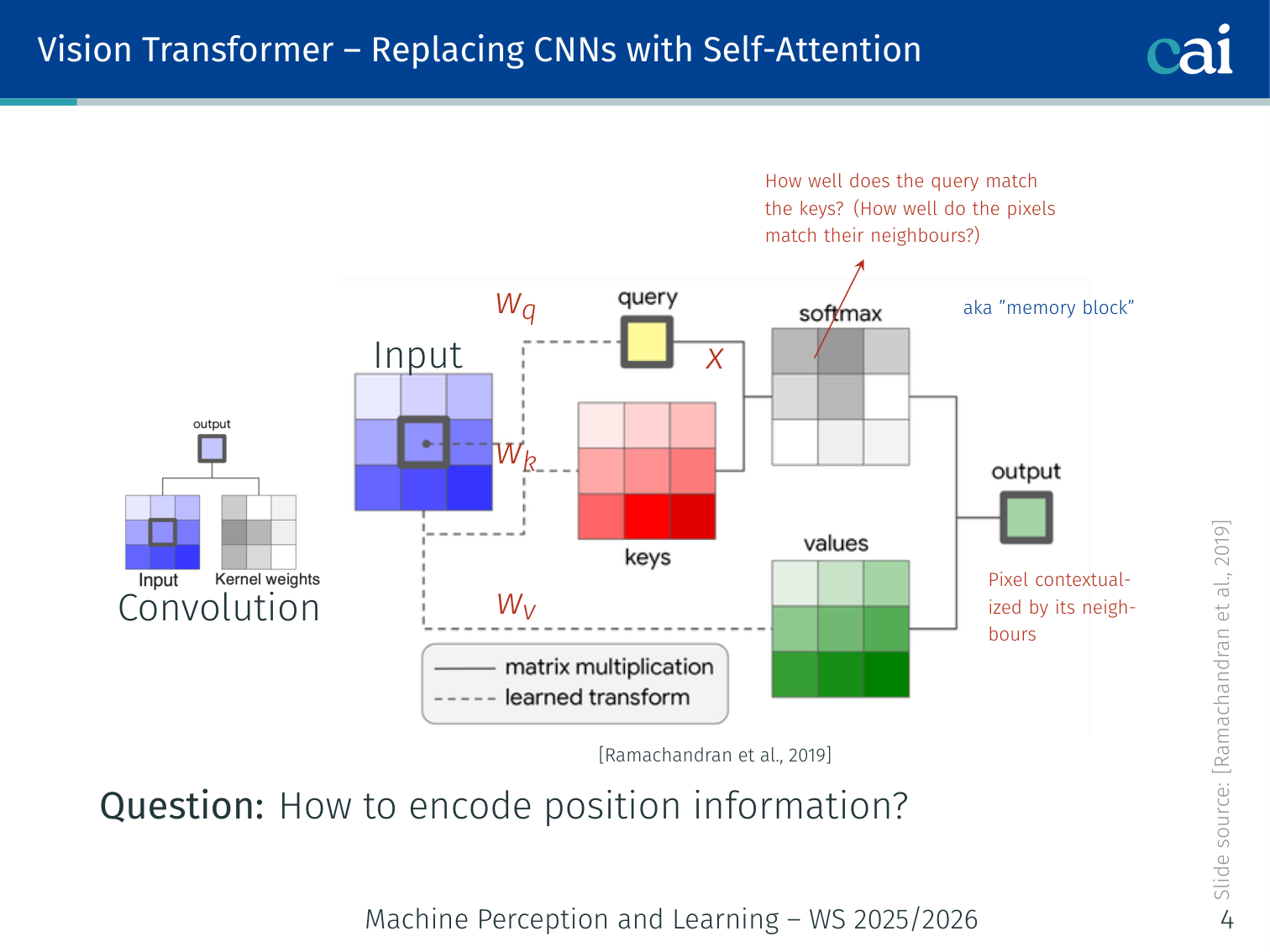
What if we just used self-attention instead of convolution? It actually works.

Before the full ViT, Ramachandran et al. (2019) showed that convolution layers can be replaced by stand-alone self-attention layers:

In a convolution, each output pixel $y_{ij}$ is a weighted sum over a local neighbourhood. In self-attention form:

$y_{ij} = \sum_{a, b \in N_{k} (i, j)} softmax_{ab} (q_{ij}^{⊤} k_{ab} + q_{ij}^{⊤} r_{a - i, b - j}) v_{ab}$

$q_{ij}$ , $k_{ab}$ , $v_{ab}$ : query, key, value projected from pixel features
$r_{a - i, b - j}$ : relative position embedding — encodes the spatial offset between $(i, j)$ and its neighbour $(a, b)$

This allows the model to ask “how well do the pixel features match their neighbours?” — just like convolution does, but with learned, data-dependent weights.

Key question: how to encode position in a 2D grid? The answer in the full ViT: add 2D position embeddings that are either fixed-sinusoidal or learned.

💡 Intuition: Why Patches? (The “Pixel vs. Word” Analogy)

In a sentence, a word is a meaningful unit. In an image, a single pixel is almost meaningless.

If we fed every pixel into a Transformer, a 224x224 image would have 50,176 tokens. Because attention is $O (n^{2})$ , this would be impossible to compute ( $50, 17 6^{2} \approx 2.5 billion$ operations per layer!).

The Solution: By grouping pixels into 16x16 patches, we treat each patch like a “word”. Now we only have 196 tokens, which is a sequence length Transformers can handle easily.

🧠 Deep Dive: The Data-Inductive Bias Tradeoff

Why do CNNs beat ViT on small datasets, but ViT wins on huge datasets?

Inductive Bias (The “Cheat Code”): CNNs “know” that images have local structure (pixels near each other are related) and that a cat is a cat whether it’s on the left or right (translation equivariance). This knowledge is a “cheat code” that helps the model learn faster with less data.
The Transformer “Tabula Rasa”: ViT starts with almost no assumptions. It doesn’t even know that patches are arranged in a grid! It has to learn the spatial relationships from scratch.
The Result: On a small dataset (ImageNet-1K), the “cheat code” (CNN) wins. But on a massive dataset (JFT-300M), the assumptions of the CNN actually become a limitation. The Transformer, free of those assumptions, can learn more complex, flexible representations that eventually surpass the CNN.

Vision Transformer (ViT) — Main Workflow

Step 1 of the ViT workflow: break the image into a sequence of small patches.

Step 2: feed those patches into a standard Transformer encoder, just like words in a sentence.

Paper: Dosovitskiy et al. “An Image is Worth 16×16 Words: Transformers for Image Recognition at Scale.” ICLR 2021.

The ViT processes images as a sequence of fixed-size patches fed into a standard Transformer encoder.

Step 1: Image Patch and Position Embedding

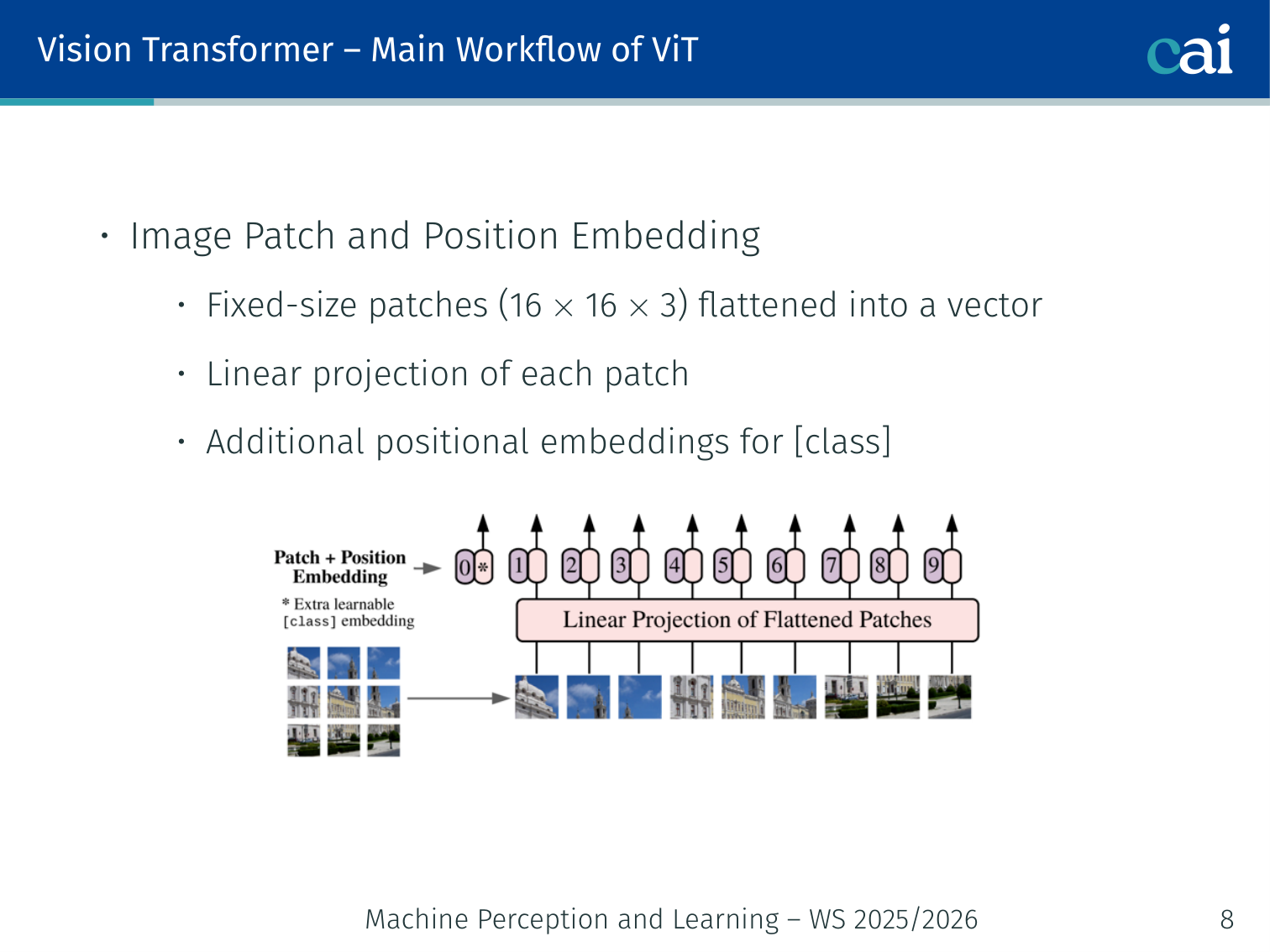
Here's a closer look at how we extract patches and add those crucial positional embeddings.

Split the image into fixed-size 16×16 patches (or 32×32) and flatten each patch into a vector
Apply a linear projection to map each flattened patch to $d_{m o d e l}$ dimensions
Add learnable positional embeddings (one per patch position)
Prepend a learnable [CLS] token — its final representation is used for classification

For a 224×224 image with 16×16 patches:

Number of patches: $(224/16)^{2} = 196$
Flattened patch size: $16 \times 16 \times 3 = 768$
Sequence length fed to Transformer: $196 + 1 = 197$ (patches + [CLS])

Example — patchifying a photo: a 224×224 RGB image of a dog becomes 196 patch tokens. Some tokens mostly contain grass, some contain the dog’s face, and others contain background sky. After patchification, the Transformer reasons over a 197-token sequence ([CLS] + 196 patches), not over the original pixel grid directly.

Image (224×224×3)
    ↓ split into non-overlapping 16×16 patches
196 patches, each 768-dimensional
    ↓ linear projection
196 tokens, each d_model=768
    ↓ prepend [CLS] token + add positional embeddings
197 tokens of dimension 768

Step 2: Encoding and Classification

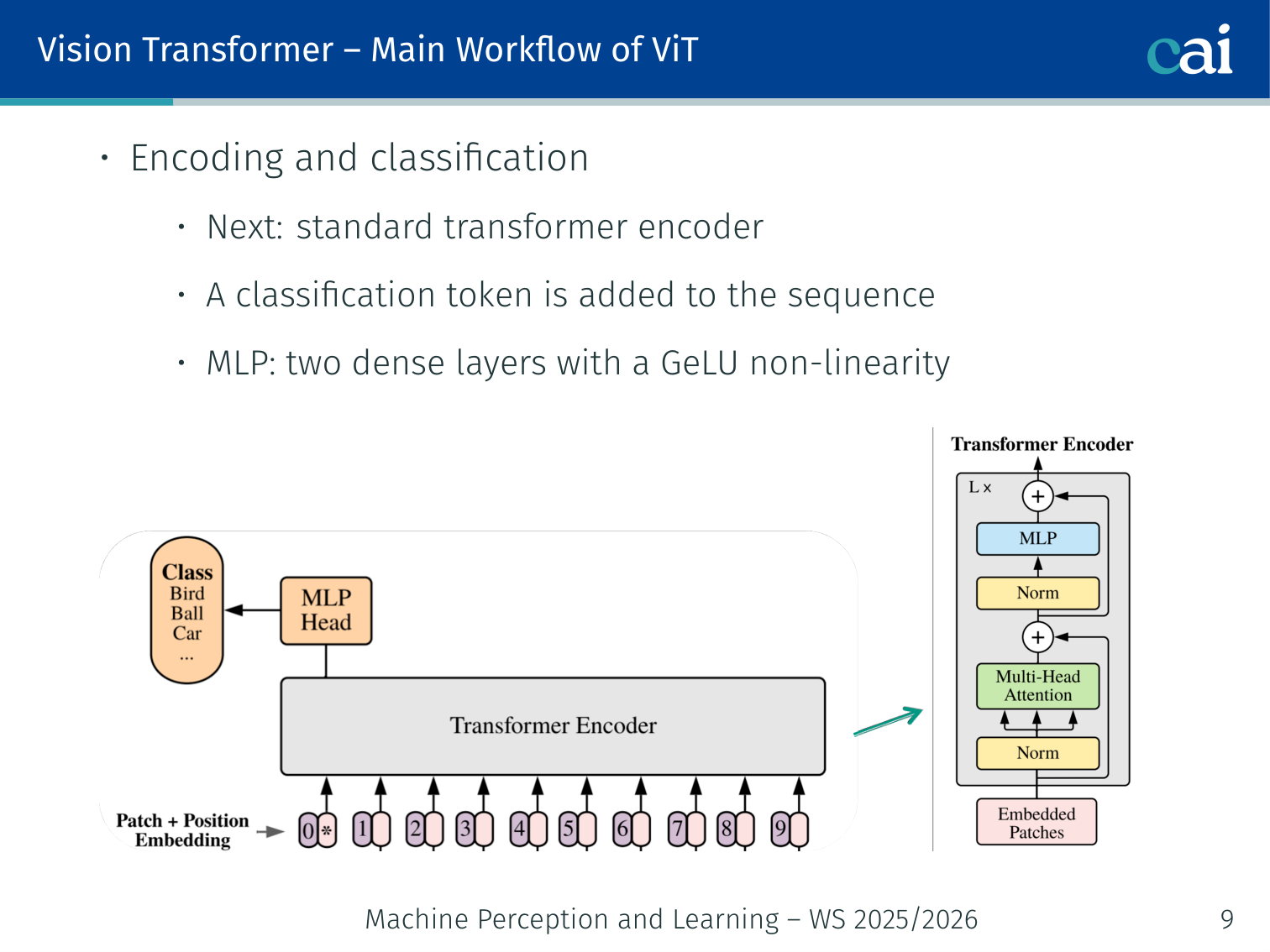
Step 2: Transformer encoding and [CLS] token classification

Feed the 197-token sequence into a standard Transformer encoder (same architecture as L05)
MLP head: two dense layers with GeLU non-linearity (not ReLU — GeLU is smoother and empirically better for ViT)
Use the [CLS] token output to make the final class prediction

197 tokens → [Transformer Encoder × L layers] → [CLS] output → [MLP head] → class logits

Why [CLS]? The [CLS] token has no patch-specific meaning — it aggregates global information from all patches via attention over all layers. This idea is borrowed directly from BERT.

ViT Architecture Versions

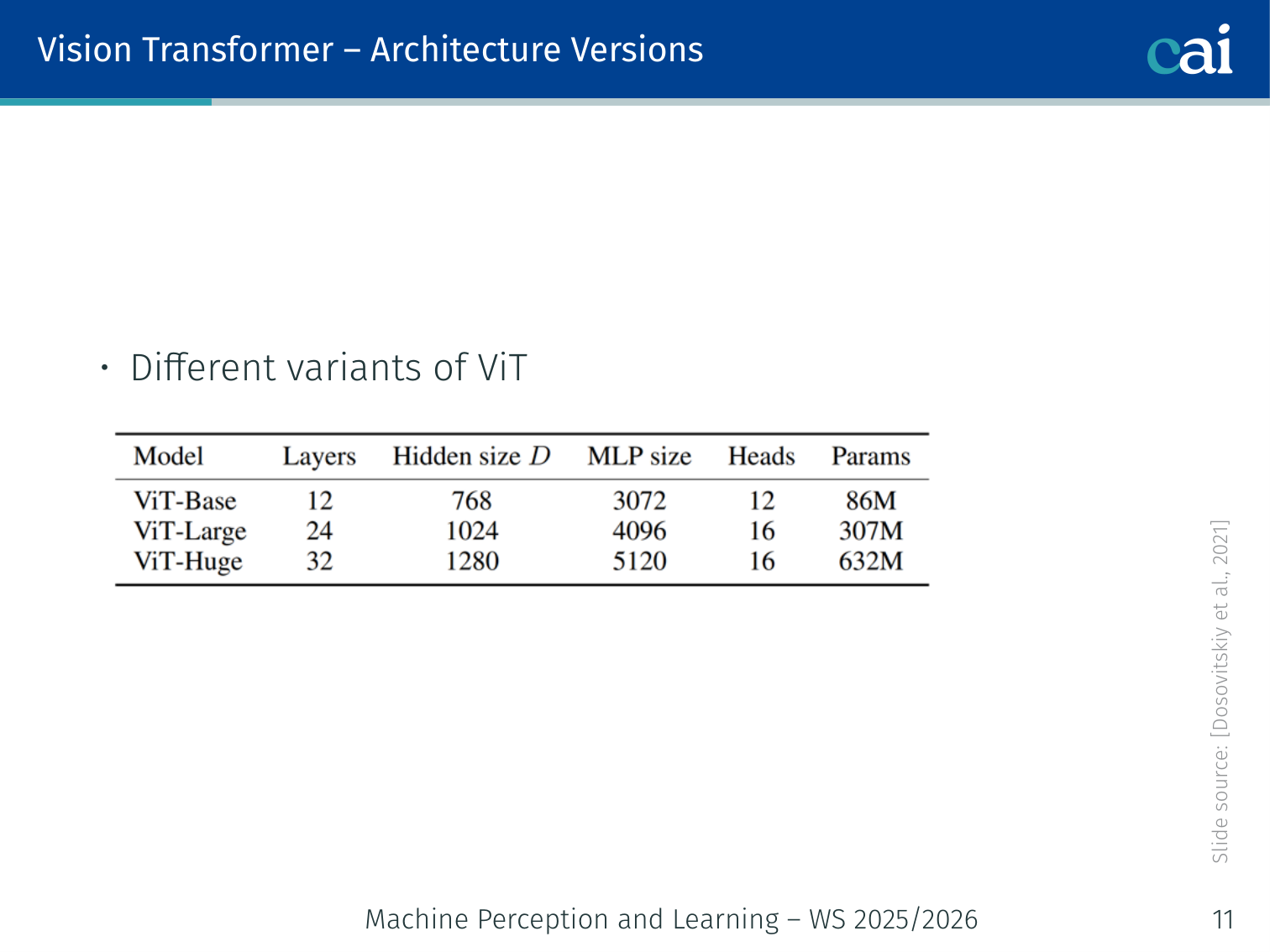
Comparison of ViT-Base, ViT-Large, and ViT-Huge configurations

Three standard variants (Dosovitskiy et al., 2021):

Model	Layers	Hidden size $d$	MLP size	Heads	Params
ViT-Base	12	768	3072	12	86M
ViT-Large	24	1024	4096	16	307M
ViT-Huge	32	1280	5120	16	632M

Both 16×16 and 32×32 patch sizes are used. Smaller patches = more tokens = more compute but better fine-grained features.

Data Requirements

ViT performance vs data scale: ImageNet-1K to JFT-300M

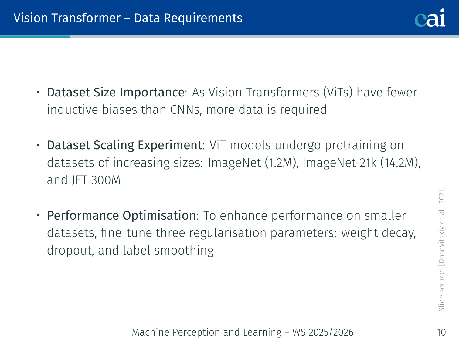
ViTs have fewer inductive biases than CNNs (no built-in locality or translation equivariance) — so they require more data to learn these structures from scratch.

Dataset scaling experiment (Dosovitskiy et al., 2021):

Pre-training dataset	Size	ViT-L vs ResNet
ImageNet-1K	1.2M images	ViT-L underperforms ResNets
ImageNet-21K	14.2M images	ViT-L ≈ ViT-B (comparable)
JFT-300M	300M images	ViT-L outperforms all ResNets

Key findings:

With ImageNet-1K only, larger ViT models (ViT-L) actually underperform smaller ones (ViT-B), even with regularisation — not enough data
The full advantage of model scale only emerges with JFT-300M pre-training
ResNets show better performance on smaller pre-training datasets, but reach a plateau earlier
ViTs benefit more from larger datasets and eventually surpass ResNets
For smaller model sizes, hybrids (CNN backbone + Transformer) outperform pure Transformers; the gap vanishes at larger scales

To improve performance on smaller datasets, three regularisation parameters help: weight decay, dropout, and label smoothing.

Example — small-data regime vs. large-data regime: on a modest dataset with only tens of thousands of labeled images, a ResNet often wins because locality and translation equivariance are built in. On web-scale pre-training data, a ViT can learn those priors from data and eventually surpass the CNN.

Attention Maps

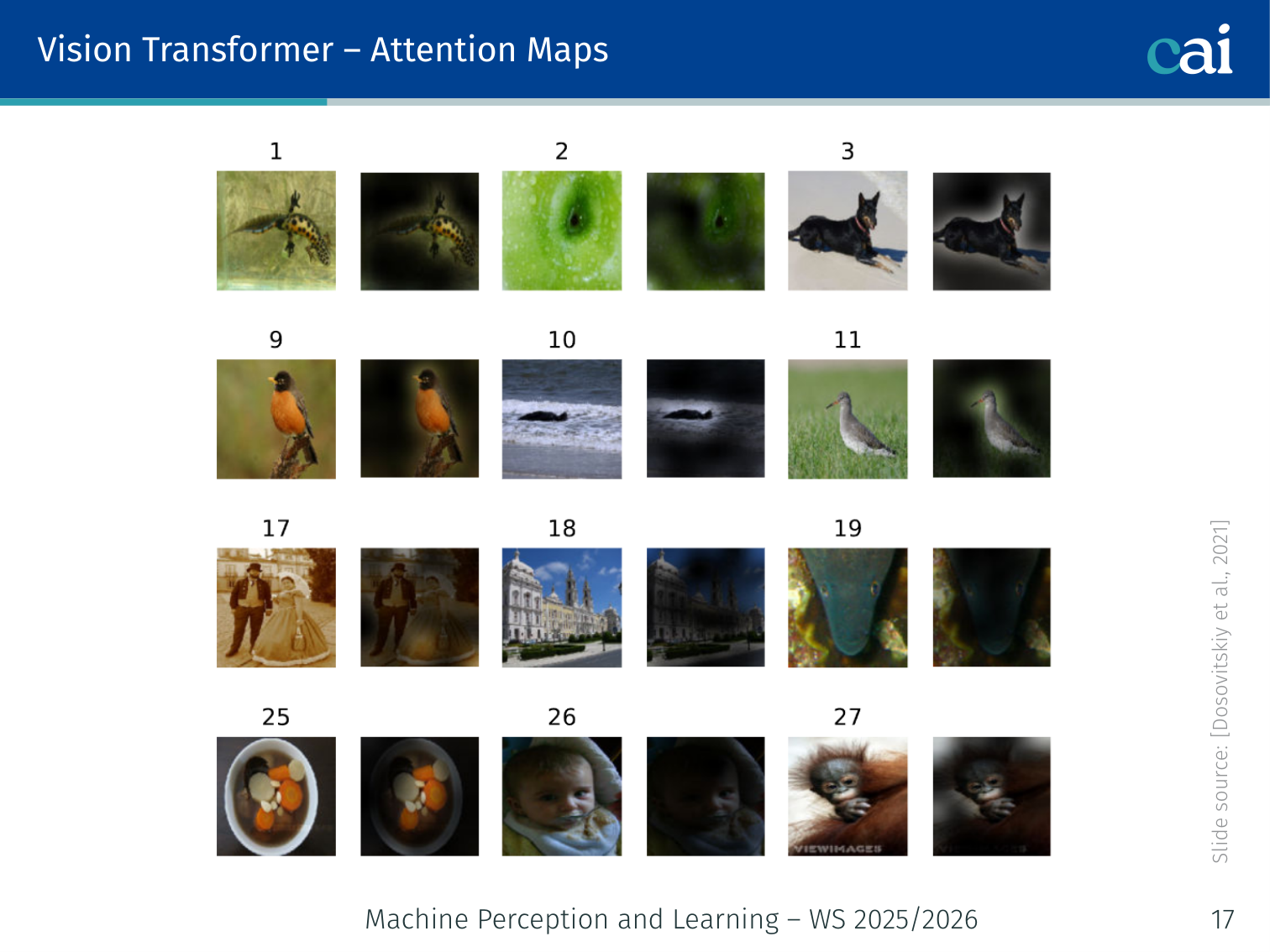
Emergent attention maps in ViT highlighting semantic objects

ViT attention maps reveal what the model “looks at” when classifying an image. Visualization of last-layer [CLS] attention weights shows:

The model attends to semantically meaningful regions — e.g., in a dog image, the [CLS] token attends to the dog’s face and body while ignoring background
This emerges without any segmentation supervision — purely from classification training
Different attention heads focus on different object parts

This is one of the most striking properties of ViT: it independently learns to segment the relevant object through the classification objective alone.

Code: ViT Patch Embedding

import torch
import torch.nn as nn
 
class PatchEmbedding(nn.Module):
    """Split image into patches and project each to d_model dimensions."""
    def __init__(self, img_size=224, patch_size=16, in_channels=3, embed_dim=768):
        super().__init__()
        self.num_patches = (img_size // patch_size) ** 2
        # Conv2d with kernel=stride=patch_size extracts non-overlapping patches
        self.proj = nn.Conv2d(in_channels, embed_dim,
                              kernel_size=patch_size, stride=patch_size)
 
    def forward(self, x):
        # x: (B, 3, 224, 224)
        x = self.proj(x)        # (B, 768, 14, 14)
        x = x.flatten(2)        # (B, 768, 196)
        x = x.transpose(1, 2)  # (B, 196, 768)
        return x
 
class SimpleViT(nn.Module):
    def __init__(self, img_size=224, patch_size=16, num_classes=1000,
                 embed_dim=768, depth=12, num_heads=12):
        super().__init__()
        num_patches = (img_size // patch_size) ** 2
 
        self.patch_embed = PatchEmbedding(img_size, patch_size, 3, embed_dim)
        self.cls_token = nn.Parameter(torch.zeros(1, 1, embed_dim))
        self.pos_embed = nn.Parameter(torch.zeros(1, num_patches + 1, embed_dim))
 
        encoder_layer = nn.TransformerEncoderLayer(
            d_model=embed_dim, nhead=num_heads,
            dim_feedforward=embed_dim * 4,  # 4× expansion (3072 for ViT-B)
            activation='gelu',              # GeLU, not ReLU
            batch_first=True
        )
        self.transformer = nn.TransformerEncoder(encoder_layer, num_layers=depth)
        self.norm = nn.LayerNorm(embed_dim)
        # MLP head: two layers with GeLU (simplified here to one linear)
        self.head = nn.Linear(embed_dim, num_classes)
 
    def forward(self, x):
        B = x.shape[0]
        x = self.patch_embed(x)                         # (B, 196, 768)
 
        # Prepend [CLS] token
        cls = self.cls_token.expand(B, -1, -1)          # (B, 1, 768)
        x = torch.cat([cls, x], dim=1)                  # (B, 197, 768)
        x = x + self.pos_embed                          # add position embeddings
 
        x = self.transformer(x)                         # (B, 197, 768)
        x = self.norm(x)
 
        # Use only the [CLS] token output for classification
        cls_out = x[:, 0]                               # (B, 768)
        return self.head(cls_out)                       # (B, num_classes)
 
# Example usage
model = SimpleViT(num_classes=1000)
img = torch.randn(4, 3, 224, 224)
logits = model(img)  # (4, 1000)

Object Detection with ViTs

Recap: CNN-Based Object Detection

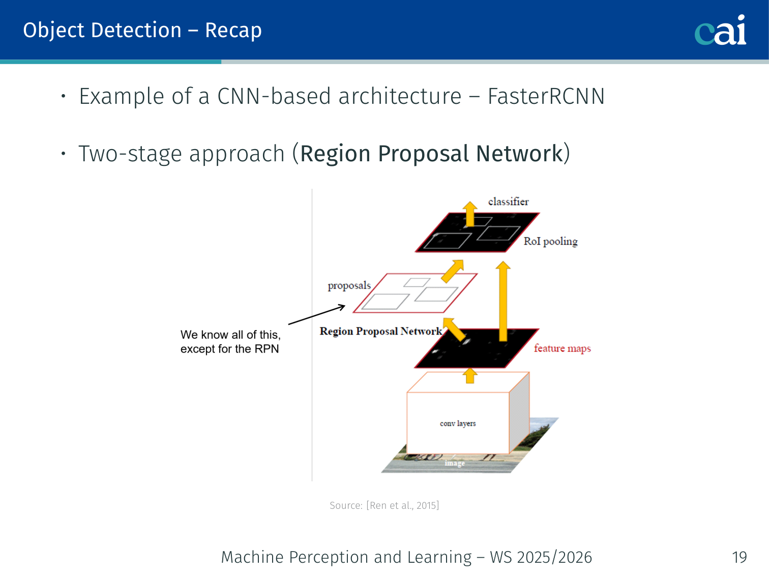
Recap of CNN-based object detection: R-CNN to Faster R-CNN

Object detection requires:

Localisation: bounding box per instance $(x, y, width, height)$
Classification: class label per bounding box (e.g., “cat”, “tv”)

CNN workflow (Faster R-CNN — Ren et al., 2015):

Region Proposal Network (RPN): generates candidate bounding boxes
ROI Pooling: extract fixed-size features for each proposed region
Classification + BBox regression: classify each ROI and refine the box
Non-Maximum Suppression (NMS): remove duplicate overlapping boxes
Introduces multi-stage processing and many hand-crafted hyperparameters

DETR — End-to-End Object Detection with Transformers

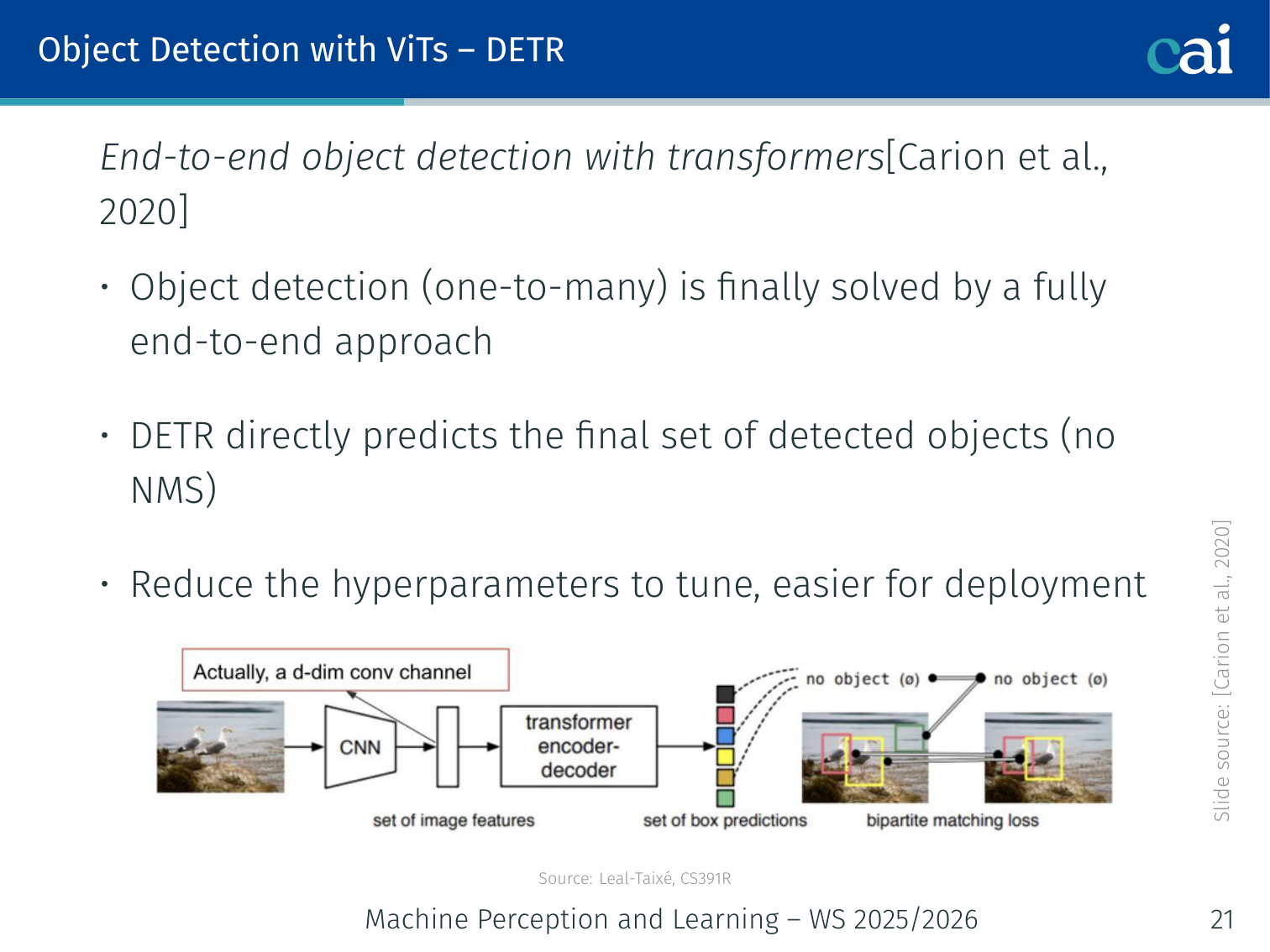
DETR: End-to-end object detection using Transformers

Paper: Carion, Massa, Synnaeve, Usunier, Kirillov, Zagoruyko. “End-to-End Object Detection with Transformers.” ECCV 2020.

Key innovation: DETR is the first fully end-to-end object detector — no RPN, no NMS, no anchor boxes. It directly predicts the final set of detected objects.

Advantages:

Eliminates hand-crafted components → fewer hyperparameters to tune
Simpler to deploy
Naturally handles one-to-many detection via set prediction

DETR Architecture

Image → [CNN Backbone] → feature map (H/32 × W/32 × 2048)
                ↓ flatten to 1D + positional encoding
         H×W sequence of spatial tokens
                ↓
         [Transformer Encoder] — self-attention over all spatial positions
                ↓
         [Transformer Decoder] ← N learnable object queries (e.g. N=100)
                ↓
         N output embeddings
                ↓ shared FFN per query
         N predictions: (class | ∅, bounding box)

Components:

CNN Backbone: extracts rich spatial features (e.g., ResNet-50); very similar to Faster R-CNN’s backbone
Positional Encoding: added to the flattened feature map before the encoder
Transformer Encoder: applies self-attention over all spatial positions — allows the encoder to separate individual instances (the encoder learns to disentangle overlapping objects)
Object Queries: $N$ learnable positional embeddings fed to the decoder. Each query specialises for a different role/location (e.g., query 3 might specialise for large objects on the left)
Transformer Decoder: cross-attends from object queries to encoder output. Qualitative finding: decoder attention typically focuses on object extremities (legs, heads, tails)
FFN heads: each query produces either a class prediction + bounding box, or a “no object” ( $\emptyset$ ) class

vs. “Attention is All You Need”: DETR’s architecture is very similar, with modifications for object detection — mainly the addition of object queries and the set-matching loss.

Optimal Bipartite Matching

Optimal bipartite matching in DETR using the Hungarian algorithm

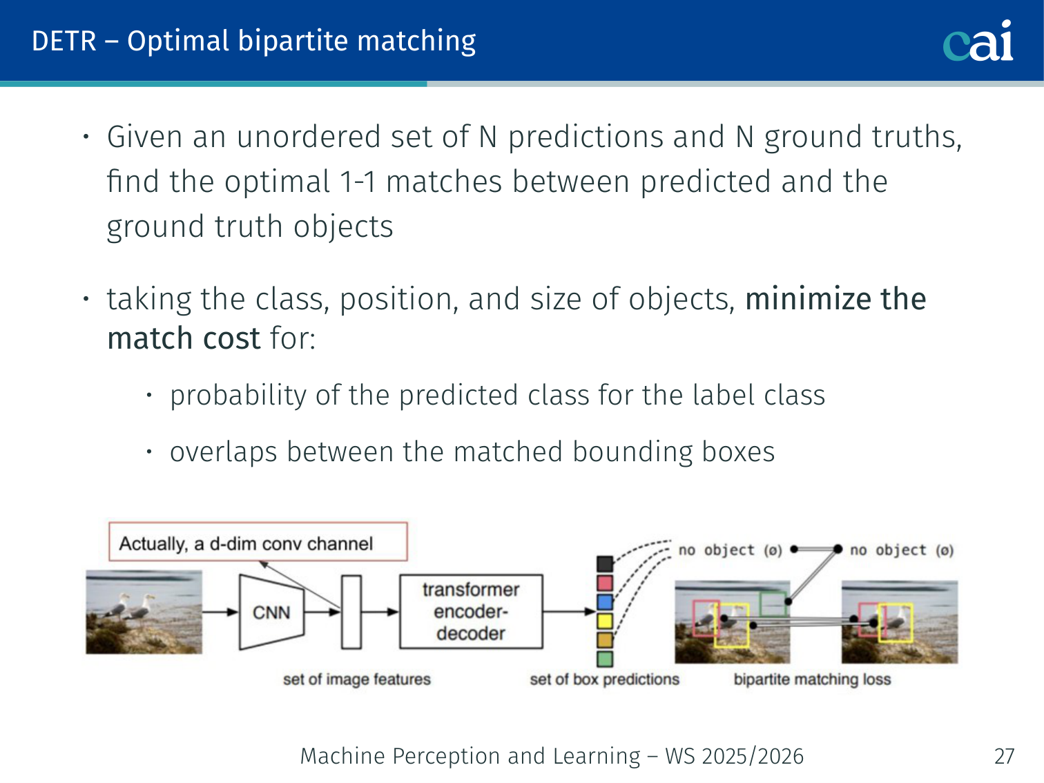
During training, $N$ predictions must be matched to the (usually fewer) ground-truth objects. DETR solves this with optimal bipartite matching:

Given an unordered set of $N$ predictions and padded ground truth $y$ , find the optimal permutation $\overset{σ}{^}$ :

$\overset{σ}{^} = ar g min_{σ \in S_{N}} \sum_{i = 1}^{N} L_{match} (y_{i}, \overset{y}{^}_{σ (i)})$

The matching cost $L_{match}$ considers:

Probability of the predicted class for the true label class
Overlap between the matched bounding boxes (IoU)

This is solved efficiently using the Hungarian algorithm (also used in Stewart et al. [2016] for people detection in crowded scenes).

Key benefit: unlike NMS, the matching is unique — every ground-truth object is matched to exactly one prediction.

Example — one dog, one bicycle, four queries: suppose an image contains one dog and one bicycle, but DETR outputs four slots: dog (0.93), bicycle (0.88), dog duplicate (0.81), and empty (0.97). Hungarian matching assigns one slot to the dog and one to the bicycle; the duplicate dog prediction is matched to $\emptyset$ and explicitly penalized during training.

Combined Loss Function (Hungarian Loss)

DETR Hungarian loss combining classification and box regression

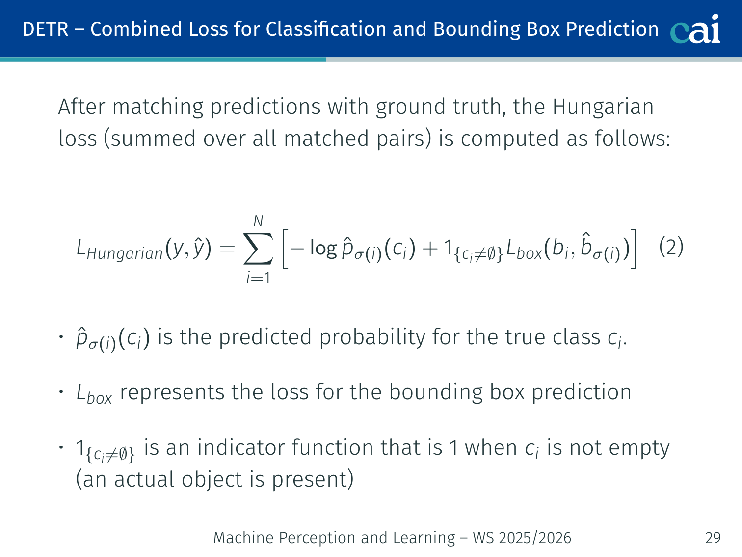
After matching, the loss over all $N$ matched pairs:

$L_{Hungarian} (y, \overset{y}{^}) = \sum_{i = 1}^{N} [- lo g \overset{p}{^}_{\overset{σ}{^} (i)} (c_{i}) + 1_{{c_{i} \neq = \emptyset}} L_{box} (b_{i}, \hat{b}_{\overset{σ}{^} (i)})]$

$\overset{p}{^}_{\overset{σ}{^} (i)} (c_{i})$ : predicted probability for the true class $c_{i}$
$L_{box}$ : bounding box regression loss (L1 + GIoU)
$1_{{c_{i} \neq = \emptyset}}$ : only compute box loss when a real object is present (not for $\emptyset$ predictions)

Example: if $N = 100$ queries but only 3 real objects in the image, 97 predictions are matched to $\emptyset$ and contribute only classification loss (predicting “no object”).

Panoptic Segmentation

Panoptic segmentation extension for DETR using a mask head

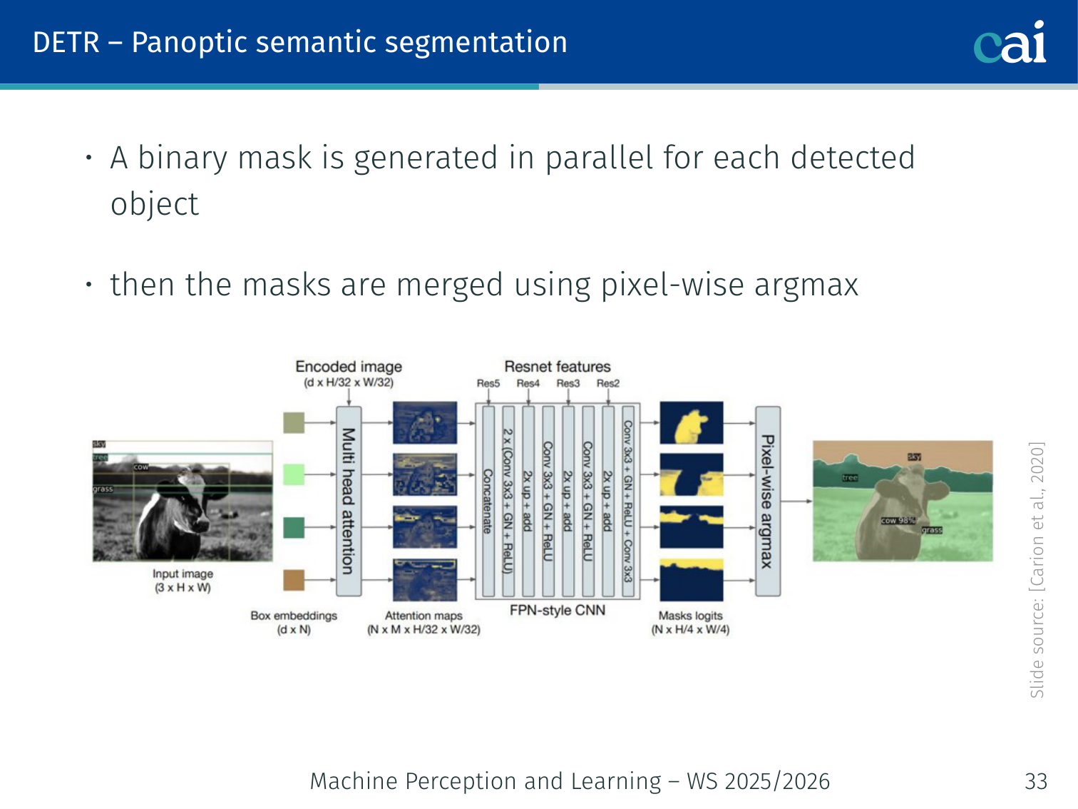
With a minor modification, DETR produces panoptic segmentation (both “things” — countable objects — and “stuff” — amorphous regions like sky, grass):

Keep the standard DETR detection head
Add a binary mask head per detected object — generates a mask in parallel
Merge all masks using pixel-wise argmax

This shows the modularity of the Transformer-based approach — segmentation requires only an additional mask branch.

DETR — Results and Shortcomings

On COCO, DETR is not just conceptually elegant; it is also competitive with strong Faster R-CNN baselines. In the lecture comparison table:

DETR-R50 reaches 42.0 AP, essentially matching Faster R-CNN-FPN at 42.0 AP
The strongest DETR variant shown, DETR-DC5-R101, reaches 44.9 AP, 64.7 AP50, and 62.3 AP_L
The weakness is visible on small objects: AP_S = 23.7, below the stronger Faster R-CNN multi-scale baseline (27.2)

The qualitative slides explain why DETR feels different from proposal-based detectors:

The encoder can separate nearby instances into different slots even in crowded scenes
The decoder often attends to object extremities such as heads, legs, and tails rather than box centers, yet still predicts coherent boxes

Shortcomings:

Problem	Cause
Slow convergence	Initially, attention weights are nearly uniform — many epochs needed before queries learn to focus on relevant locations
Poor small object detection	Full-resolution attention is $O (n^{2})$ — hard to use high-resolution feature maps without prohibitive cost

Deformable DETR (Zhu et al., 2020)

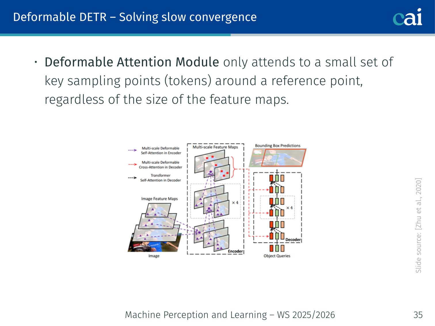
Deformable DETR: sparse attention for faster convergence

Two targeted fixes for DETR’s shortcomings:

1. Deformable Attention Module — solves slow convergence:

Instead of attending to all spatial tokens, each query attends to only a small set of key sampling points around a reference point (typically 4 per head)
Cost is dramatically reduced regardless of feature map size
Attention focuses quickly on relevant locations

2. Multi-scale Deformable Attention — solves small object detection:

Looks over sampling points from multi-scale feature maps simultaneously (e.g., 1/8, 1/16, 1/32, 1/64 of input resolution)
Small objects are better represented at finer scales
Uses CNN-style FPN-like multi-scale features

Result: Deformable DETR converges ~10× faster than DETR and significantly improves small object AP.

Example — far-away traffic sign: in a street scene, a distant stop sign may occupy only a tiny region. Vanilla DETR spreads attention across the whole feature map, so that signal is weak. Deformable DETR samples a handful of relevant points on fine-resolution features near the sign, making the query lock onto it much faster.

# Conceptual: deformable attention samples K points per head
# instead of attending to all H×W positions
# reference_point: (B, Q, 2) — normalized grid coordinates per query
# sampling_offsets: (B, Q, num_heads, K, 2) — learned offsets per head
# attention_weights: (B, Q, num_heads, K) — weights over sampled points

Self-supervised Vision Transformers

Motivation

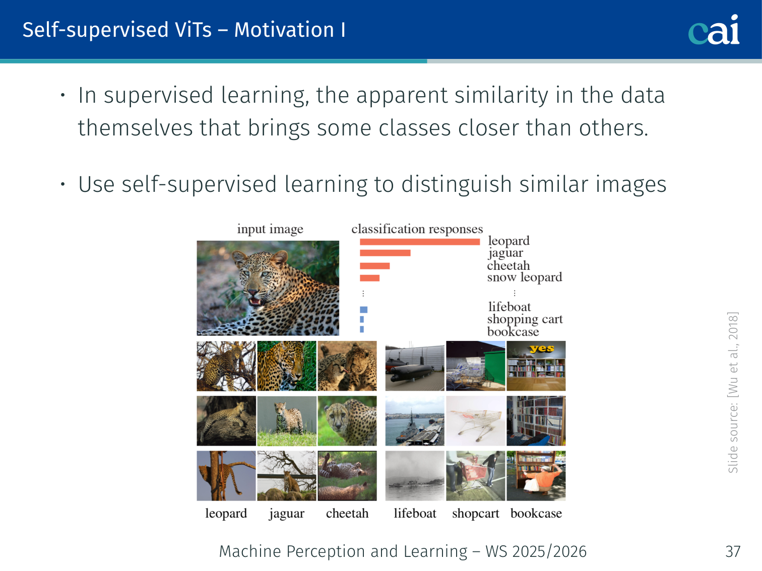
Motivation for self-supervised visual representation learning

Supervised learning challenge: when labeled examples are clustered in feature space by their label, their apparent similarity is determined by the labels themselves — not by genuine visual similarity.

Self-supervised goal: learn representations that distinguish visually similar images even without labels.

Why now? Transformers drove NLP progress through self-supervised learning (BERT, GPT) — can the same approach work for vision? Vision Transformer (ViT, L06) was trained in a fully supervised manner — we want to explore self-supervised alternatives.

Pretext Tasks in NLP

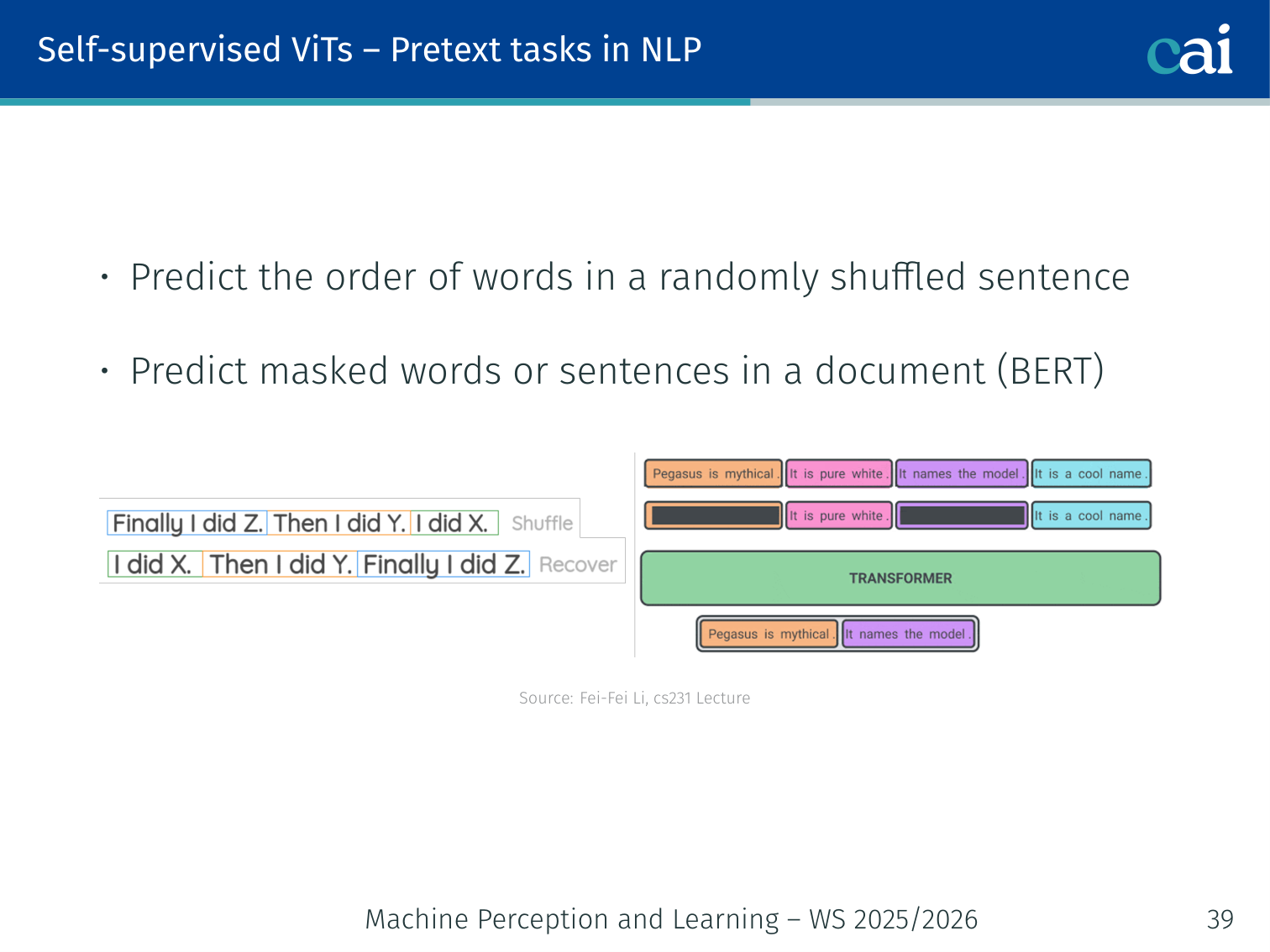
Analogous pretext tasks in NLP: MLM and NSP

Self-supervised learning in NLP defines pretext tasks where labels come automatically from the data:

BERT (Devlin et al., 2019): predict masked words in a sentence (MLM) + next sentence prediction
GPT (Radford et al., 2019): language modelling — predict the next word left-to-right

These tasks forced the model to learn rich semantic representations without human annotation.

Pretext Tasks in Computer Vision

Visual pretext tasks: rotation prediction and jigsaw puzzles

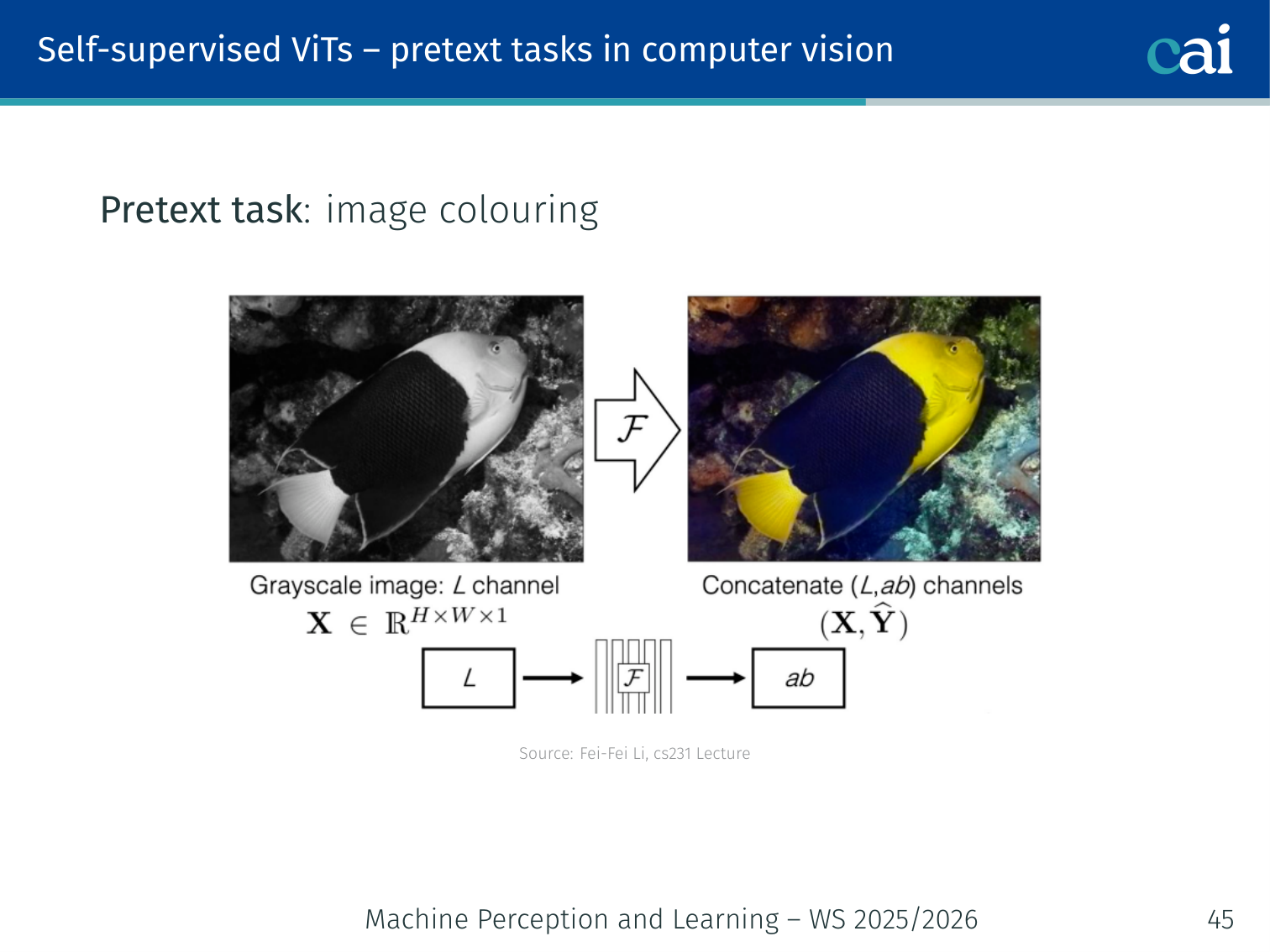
Visual pretext tasks: inpainting and colorization

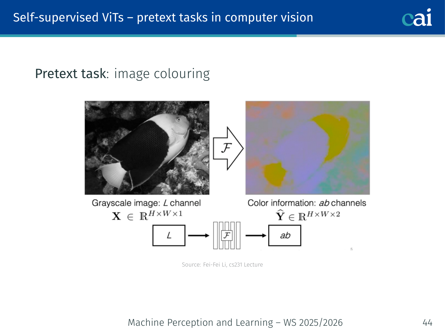
Many analogous pretext tasks were proposed for vision (Li, cs231):

Pretext Task	Hypothesis
Predict image rotation (0°, 90°, 180°, 270°)	To know the correct orientation, the model must understand what objects “should” look like
Predict relative patch location	The model must understand spatial layout and object structure
Solve jigsaw puzzles	Shuffled patches require understanding of coherent composition
Predict missing pixels (inpainting)	The model must understand context to hallucinate missing regions
Image colouring	To colour a grayscale image, the model must understand object semantics (grass is green, sky is blue)

Problem with pretext tasks: the learned representations may be tied to the specific task. A model trained to predict rotation may learn to detect horizon lines without learning object semantics. The representations don’t necessarily transfer well to downstream tasks.

Self-Supervised Contrastive Learning

Framework for self-supervised contrastive learning

An alternative to pretext tasks: contrastive learning with augmented view pairs.

Idea:

Take an image and create two different augmented views of the same image → these are positive pairs
Views of different images → negative pairs
Minimise the distance between positive pair representations
Maximise the distance from all negative pair representations

Image x ──augment_1──→ view₁ ──encoder──→ z₁
         ──augment_2──→ view₂ ──encoder──→ z₂

loss: bring z₁ and z₂ close together, push apart from all z_other

Key question: Do Transformers encode different properties than CNNs under self-supervision?

Transformers have no built-in locality (no convolutions) → no strong principle of locality is enforced
Under self-supervision, Transformers may encode scene layout or object boundaries differently
This motivated DINO (below)

DINO — Self-supervised Vision Transformers

DINO: Knowledge distillation with no labels in ViTs

Paper: Caron, Touvron, Misra, Jégou, Mairal, Bojanowski, Joulin (2021). “Emerging Properties in Self-Supervised Vision Transformers.” ICCV 2021.

Multi-Crop Strategy

DINO multi-crop strategy: local and global views

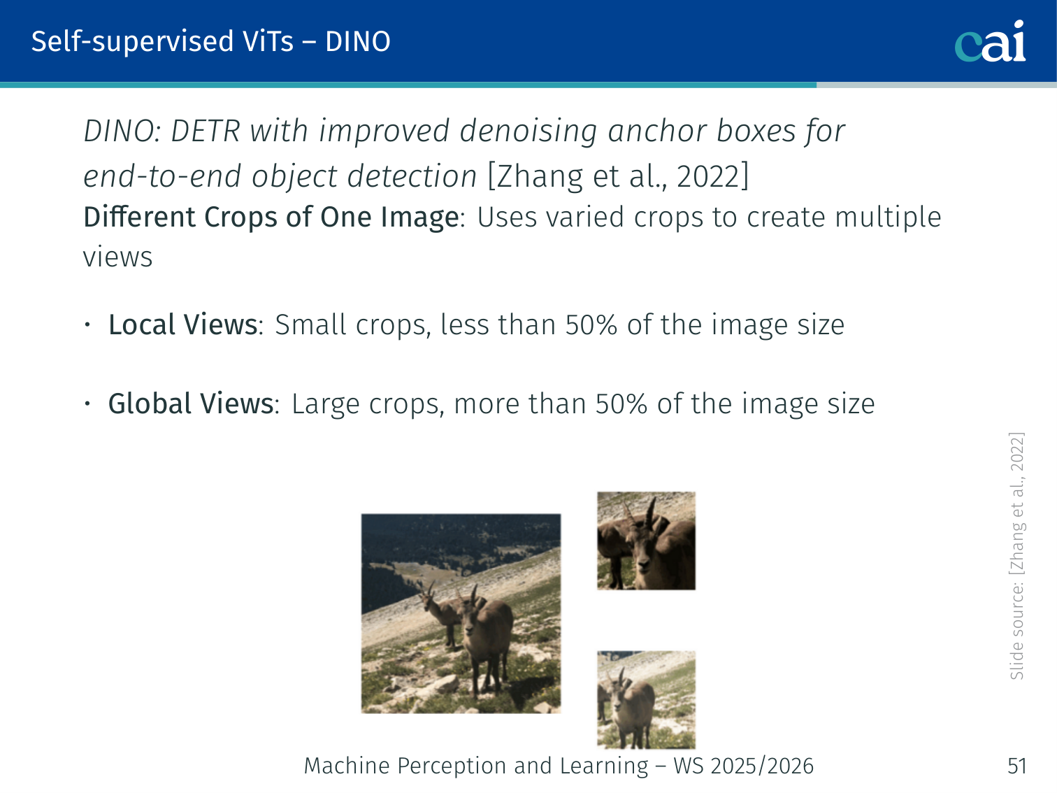
DINO uses different crops of one image to create multiple views:

Local views: small crops — less than 50% of the image area
Global views: large crops — more than 50% of the image area

This asymmetry forces the model to learn local-to-global correspondence: the student sees small local patches and must learn to match the global understanding captured by the teacher.

Example — bird image: a local crop may contain only a bird’s wing, while a global crop shows the full bird on a branch. The student must map that wing-only view to the same semantic representation that the teacher produces from the full scene.

Knowledge Distillation: Teacher-Student Framework

Teacher-student distillation framework in DINO

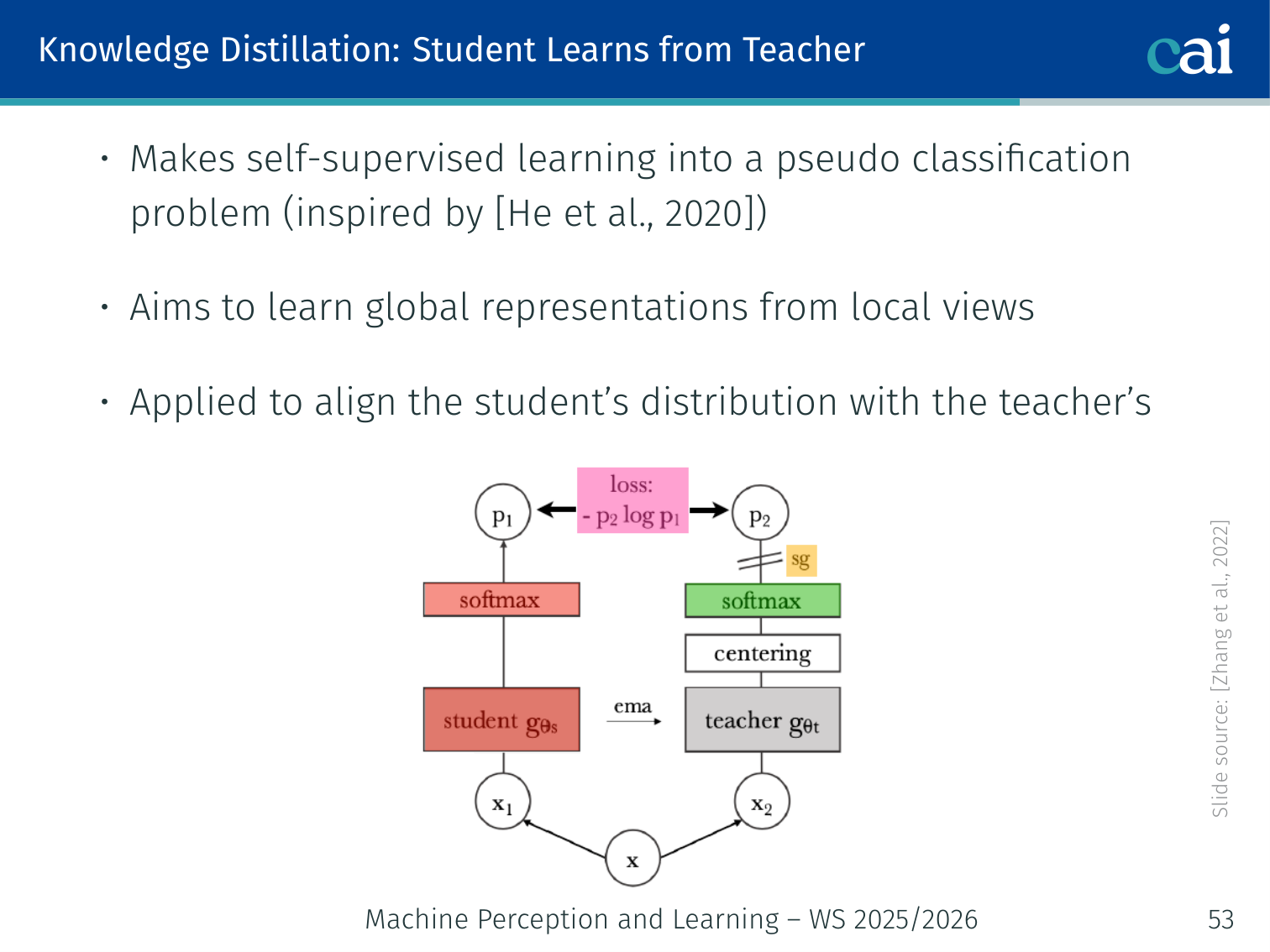
DINO frames self-supervised learning as a pseudo-classification problem via knowledge distillation (inspired by He et al. [MoCo], 2020):

Local view  → [Student ViT]  → student distribution Pₛ(x)
Global view → [Teacher ViT] → teacher distribution Pₜ(x)

Objective: minimise H(Pₜ(x), Pₛ(x))  ← student learns to match teacher

Teacher weights = exponential moving average (EMA) of student weights — no gradient flows through the teacher
The teacher sees only global views; the student sees both global and local views
This encourages the student to extrapolate from local context to global understanding

Loss Functions

Student distribution (softmax with temperature $τ_{s}$ ):

$P_{s} (x) (i) = \frac{e x p ( θ _{s} ( x ) ( i ) / τ _{s} )}{\sum _{k = 1}^{K} e x p ( θ _{s} ( x ) ( k ) / τ _{s} )}$

Teacher distribution (softmax with temperature $τ_{t}$ ):

$P_{t} (x) (i) = \frac{e x p ( θ _{t} ( x ) ( i ) / τ _{t} )}{\sum _{k = 1}^{K} e x p ( θ _{t} ( x ) ( k ) / τ _{t} )}$

$τ_{s} > 0$ , $τ_{t} > 0$ : temperature hyperparameters ( $τ_{t} < τ_{s}$ makes the teacher sharper)
$K$ : total number of output features/classes
$θ_{s}$ , $θ_{t}$ : student and teacher model parameters

Cross-entropy loss (minimised w.r.t. student parameters only):

$min_{θ_{s}} H (P_{t} (x), P_{s} (x)) where H (a, b) = - a lo g b$

Multi-view loss (over all crops):

$min_{θ_{s}} \sum_{x \in {x_{1}^{g}, x_{2}^{g}}} \sum_{x^{'} \in V x^{'} \neq = x} H (P_{t} (x), P_{s} (x^{'}))$

Only global views ${x_{1}^{g}, x_{2}^{g}}$ are passed to the teacher
All views (global + local) $V$ are passed to the student

Mode Collapse Problem

Visualization of the mode collapse problem in self-supervision

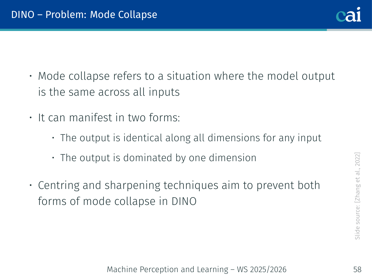
Mode collapse occurs when the model outputs the same distribution for all inputs, making the loss trivially zero:

The output is identical along all dimensions for any input
The output is dominated by a single dimension (one feature value is always highest)

Both forms result in learned representations that carry no useful information.

Centering to Prevent Mode Collapse

Centering and sharpening techniques in DINO to prevent collapse

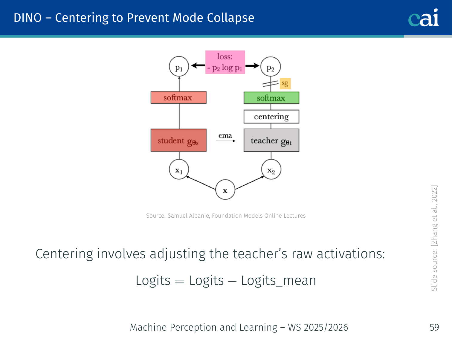
DINO prevents mode collapse with two complementary techniques:

Centering (prevents dimension dominance):

$Logits = Logits - \overline{Logits}$

Subtract a running mean from the teacher’s raw activations before the softmax:

Features that are above their mean become positive → softmax assigns high probability
Features below their mean become negative → softmax assigns low probability
Prevents any single feature from always dominating by centering the range

Sharpening (prevents uniform outputs):

Use a low teacher temperature $τ_{t}$ → sharper, more confident teacher distribution
Forces the student to commit to specific features rather than predicting a uniform distribution

Together: centering prevents one dimension from always winning; sharpening prevents everything from being equally likely.

# Conceptual DINO training loop
import torch
import torch.nn.functional as F
 
def dino_loss(student_out, teacher_out, tau_s=0.1, tau_t=0.04, center=None):
    # Center the teacher output to prevent mode collapse
    teacher_out = teacher_out - center  # subtract running mean
 
    # Compute distributions
    s = F.softmax(student_out / tau_s, dim=-1)
    t = F.softmax(teacher_out / tau_t, dim=-1)
 
    # Cross-entropy: student learns to match teacher
    loss = -(t * torch.log(s + 1e-8)).sum(dim=-1).mean()
    return loss
 
# Teacher is updated via EMA of student weights (no gradient)
# for param_t, param_s in zip(teacher.parameters(), student.parameters()):
#     param_t.data = momentum * param_t.data + (1 - momentum) * param_s.data

Results

DINO is very effective for Transformer backbones:

On ResNet-50, DINO is already competitive with the best CNN self-supervised baselines in the lecture table: 75.3 linear-eval accuracy and 67.5 $k$ -NN accuracy
On ViT-S, the gains are clearer: DINO reaches 77.0 linear accuracy and 74.5 $k$ -NN, outperforming BYOL, MoCov2, and SwAV on the same Transformer backbone
Self-supervised ViTs develop explicit semantic segmentation maps in their last-layer attention — clear foreground/background separation with no segmentation labels
$k$ -NN classification on ImageNet without fine-tuning achieves strong accuracy, demonstrating the quality of learned representations
Attention maps are semantically interpretable: the model identifies object boundaries and scene structure for objects such as birds, boats, bicycles, giraffes, dogs, and even large scene regions like skylines
DINO features transfer well across datasets and tasks

Example — emergent segmentation without labels: for a dog standing on grass, the last-layer DINO attention often highlights the dog’s body as one coherent region while downweighting the background, even though the model never saw a segmentation mask during training.

These properties do not emerge as strongly in CNN-based self-supervised models — the inductive biases of Transformers (global attention, no forced locality) appear to be key.

DINO became the foundation for DINOv2, SAM (Segment Anything Model), and other prominent vision foundation models.

The Field is Evolving Quickly

Summary of the rapid evolution in vision and language models

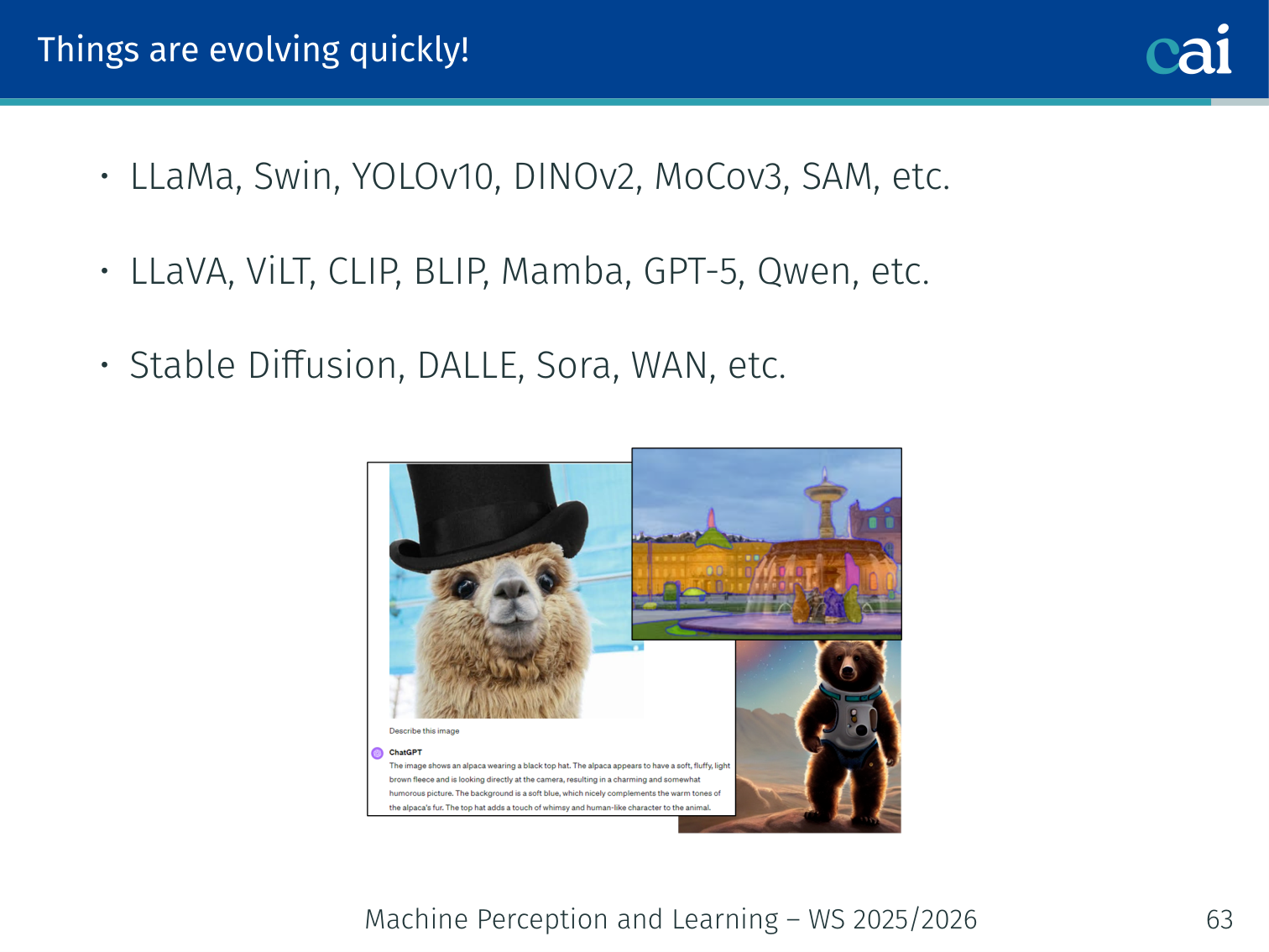
From the lecture’s closing slide — notable models and frameworks as of WS 2025/2026:

Backbone models: Swin, MoCov3, DINOv2
Detection: YOLOv10, DINO (detection variant), Deformable DETR
Vision-Language: LLaVA, ViLT, CLIP, BLIP, Qwen
Language: LLaMA, GPT-5, Mamba
Generative: Stable Diffusion, DALL-E, Sora, WAN

Summary

Topic	Key Points
CNN limitations	Brittle to certain distribution shifts; Transformers show better robustness but need explicit position encoding
Stand-alone self-attention	Can replace convolution; relative position embedding captures spatial structure
ViT	16×16 patches as tokens; [CLS] for classification; GeLU MLP head; needs large data (JFT-300M > ImageNet-21K > ImageNet-1K)
ViT data scaling	ResNets better on small datasets; ViT surpasses at JFT-300M scale
DETR	CNN backbone + Transformer encoder/decoder; $N$ object queries; Hungarian matching; no NMS; slow convergence, poor small objects
Deformable DETR	Sparse deformable attention + multi-scale features; solves DETR’s shortcomings
Pretext tasks	Rotation, jigsaw, inpainting, colouring — but representations tied to task
Contrastive learning	Positive (same image, different augmentations) vs negative pairs; minimize/maximize distance
DINO	Teacher (EMA) + student; global views to teacher only; local-to-global correspondence; centering + sharpening prevents mode collapse; emergent segmentation

References

Carion, Massa, Synnaeve, Usunier, Kirillov, Zagoruyko (2020) — End-to-end object detection with transformers. ECCV, pp. 213–229.
Dosovitskiy et al. (2021) — An image is worth 16×16 words: Transformers for image recognition at scale. arXiv:2010.11929.
He, Fan, Wu, Xie, Girshick (2020) — Momentum contrast for unsupervised visual representation learning. CVPR, pp. 9729–9738.
Naseer, Ranasinghe, Khan et al. (2021) — Intriguing properties of vision transformers. NeurIPS, 34:23296–23308.
Ramachandran, Parmar, Vaswani, Bello, Levskaya, Shlens (2019) — Stand-alone self-attention in vision models. arXiv:1906.05909.
Ren, He, Girshick, Sun (2015) — Faster R-CNN: Towards real-time object detection with region proposal networks. NeurIPS, 28:91–99.
Stewart, Andriluka, Ng (2016) — End-to-end people detection in crowded scenes. CVPR, pp. 2325–2333.
Wu, Xiong, Yu, Lin (2018) — Unsupervised feature learning via non-parametric instance discrimination. CVPR, pp. 3733–3742.
Caron, Touvron, Misra, Jégou, Mairal, Bojanowski, Joulin (2021) — Emerging properties in self-supervised vision transformers. ICCV.
Zhu, Su, Lu, Li, Wang, Dai (2020) — Deformable DETR: Deformable transformers for end-to-end object detection. arXiv:2010.04159.

Applied Exam Focus

Patch Projection: ViT treats an image as a sequence of $16 \times 16$ patches, effectively turning a Vision problem into an NLP problem.
Inductive Bias: ViT has less inductive bias than CNNs (no translation invariance or locality). This means it requires much more data to outperform CNNs.
Hybrid Models: Often use a CNN backbone to extract features before passing them to a Transformer for global reasoning.

Previous: L05 — Transformers | Back to MPL Index | Next: (y-07) Multimodal | (y) Return to Notes | (y) Return to Home

Yusuf's Thoughts

Explorer