L07 — Multimodal Learning

Previous: L06 — ViT | Back to MPL Index | Next: (y-08) IML

This lecture covers:

Motivation of Multimodal Learning
Multimodal Representation Learning
Multimodal Alignment
Multimodal Reasoning

Mental Model First

Multimodal learning is about getting very different data types to talk to each other.
The hard part is not only fusion; it is also representation, alignment, translation, and deciding when signals from different modalities agree or conflict.
Shared embedding spaces matter because they let the model compare images, text, audio, and other signals using one common geometry.
If one question guides this lecture, let it be: how do we connect heterogeneous modalities without destroying the information that makes each one useful?

1. Motivation of Multimodal Learning

What is Multimodal?

Multimodal is just combining different data types like images, audio, and text.

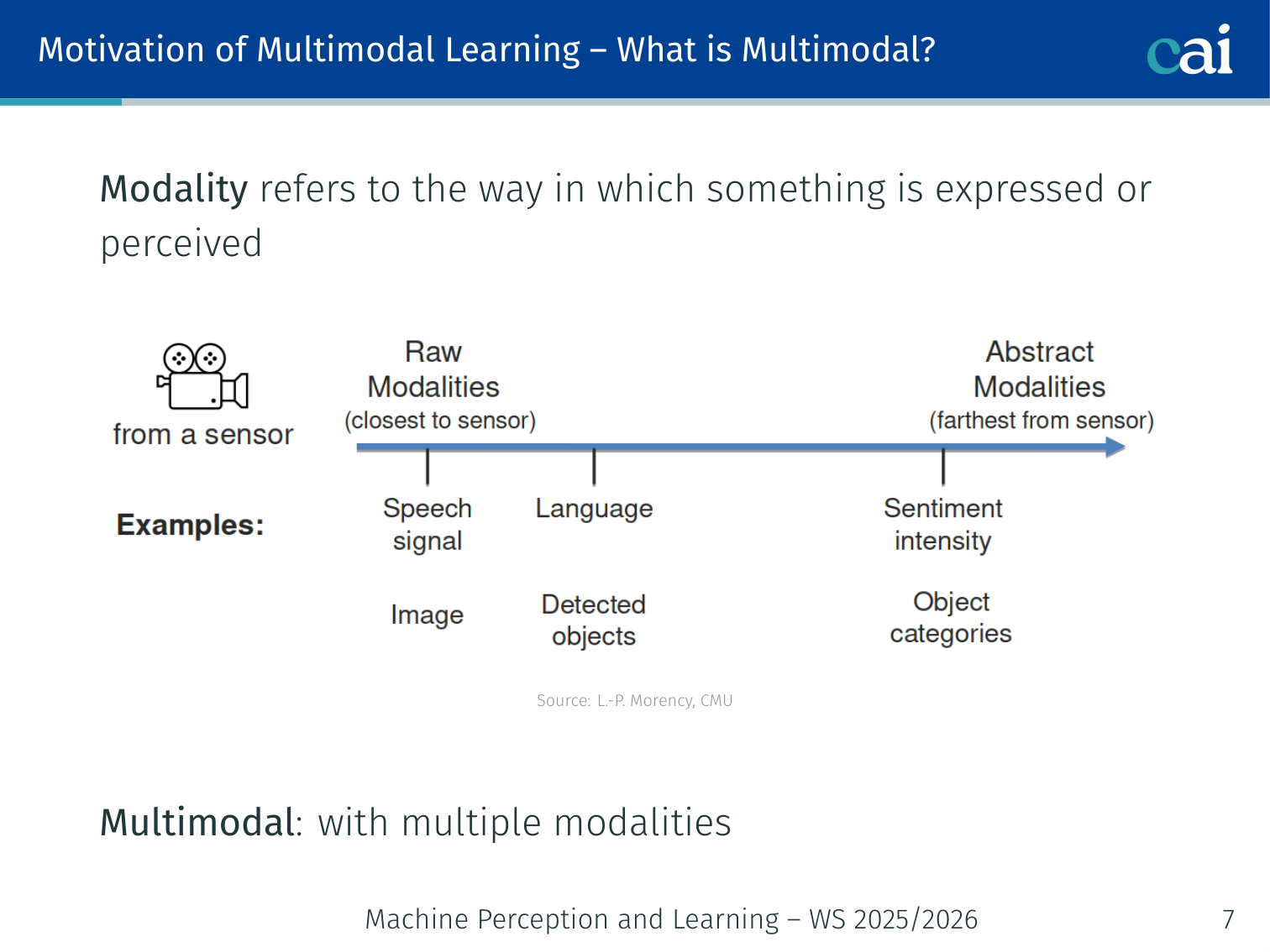
Modality refers to the way in which something is expressed or perceived (sight, sound, text, touch, …). Multimodal means using multiple modalities together.

From a probability perspective, multimodal originally means multiple modes (local maxima) in a probability density — the term was adopted by the field to describe systems that handle multiple data types.

Three definitions of increasing scope (Baltrušaitis et al., 2018 / Morency, CMU):

Term	Definition
Multimodal Machine Learning	Computer algorithms that learn and improve through the use of multimodal data
Multimodal AI	Agents that demonstrate intelligence (understanding, reasoning, planning) through multimodal experiences
Multimodal Science	Study of heterogeneous and interconnected (connected + interacting) data

Heterogeneity of Modalities

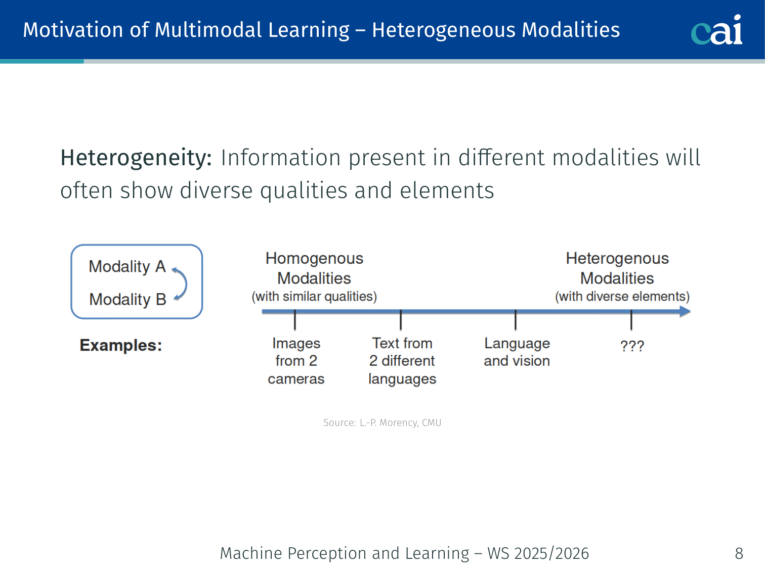
Each modality has its own structure—think dense video frames versus discrete text tokens.

Information in different modalities shows diverse qualities, structures, and noise levels:

Video: spatial + temporal, high-dimensional, dense
Speech / Audio: sequential, waveform or spectrogram
Text: symbolic, discrete, structured by grammar
Physiological signals: low-dimensional, noisy

This heterogeneity is both a challenge and an opportunity — each modality carries complementary information.

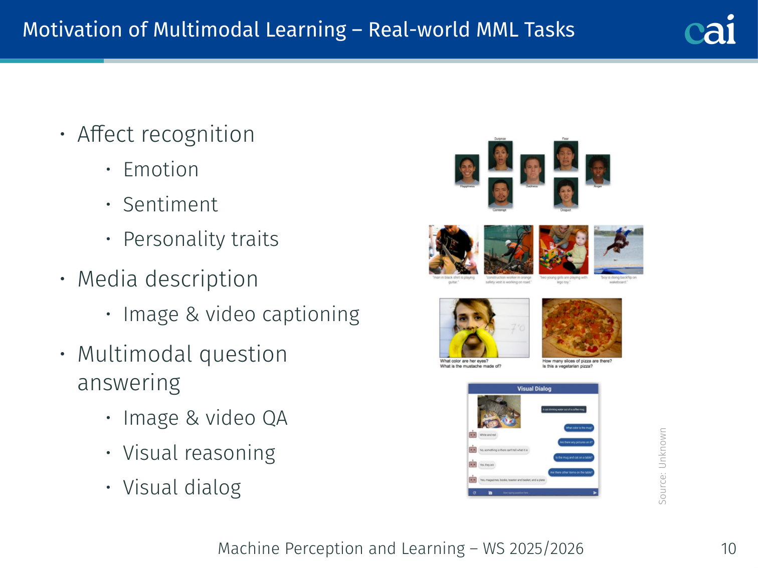
Real-World Multimodal Tasks

Here are some common tasks where you'd actually use multimodal learning.

Category	Examples
Affect recognition	Emotion, sentiment, personality from face + voice + text
Media description	Image & video captioning
Visual Q&A / Reasoning	VQA, visual dialog, multimodal QA
Navigation	Language-guided navigation, autonomous driving
Event recognition	Action recognition, segmentation
Multimedia retrieval	Content-based and cross-media search

Example — Affect recognition: given a video of someone speaking, the model uses their facial expression (vision), tone of voice (audio), and the words they say (text) to predict whether they are happy, frustrated, or neutral. Unimodal models (text-only, audio-only) perform significantly worse than fusion approaches.

2. Core Multimodal Challenges

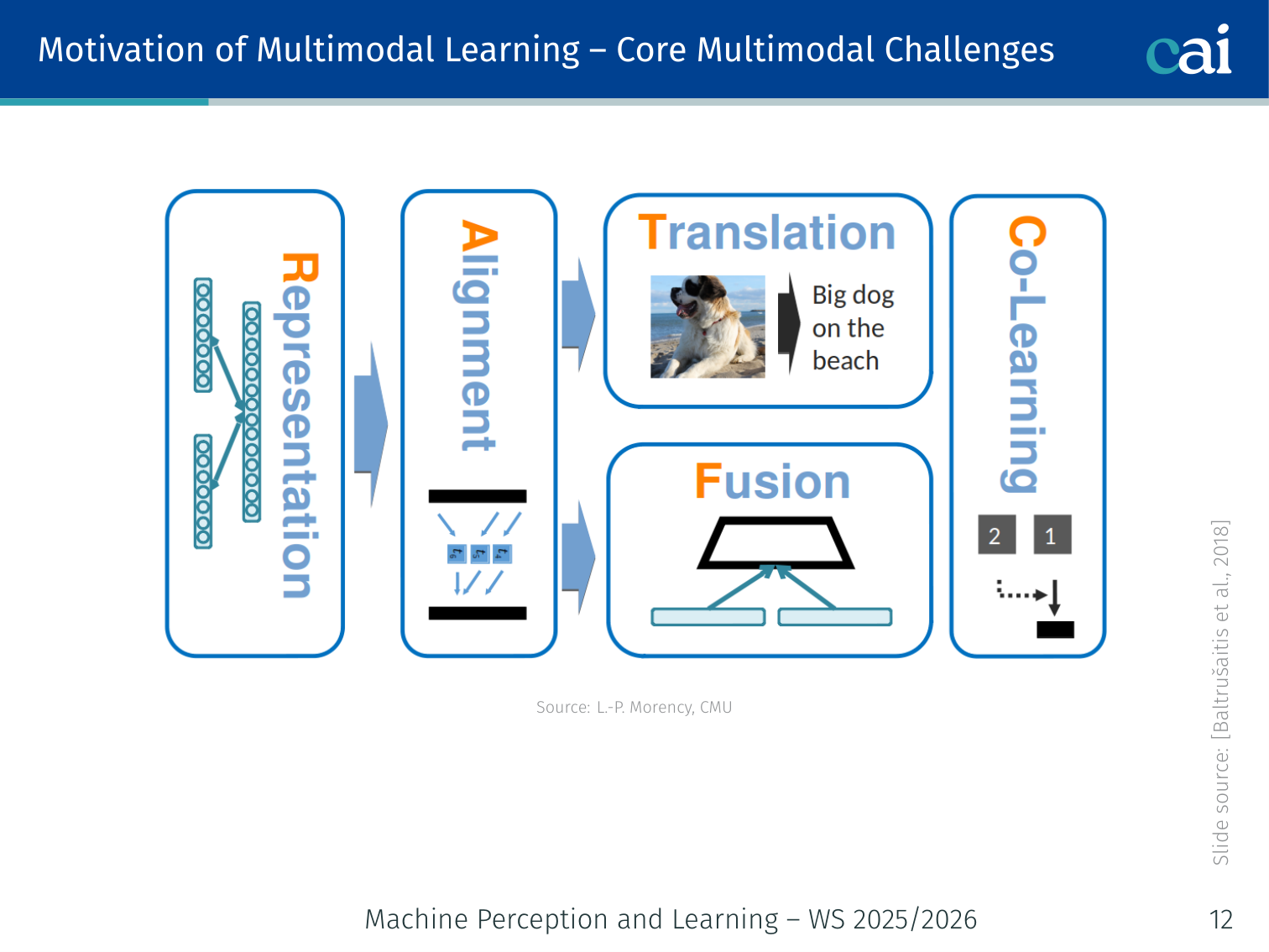
These are the five main hurdles we have to clear in multimodal ML.

Baltrušaitis et al. (2018) define five fundamental challenges for multimodal machine learning:

Challenge 1: Representation

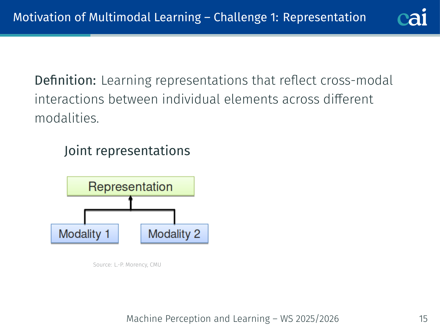
We can either fuse everything into one space or keep them separate but aligned.

Definition: Learning representations that reflect cross-modal interactions between individual elements across different modalities.

Two families:

Type	Description	Example
Joint representation	Combine modalities into a single shared space (fusion)	CLIP embedding space
Coordinated representation	Keep separate spaces but enforce a coordination constraint between them	DeViSE — image and word-vector spaces constrained by cosine similarity

Early examples:

Bimodal Deep Belief Network (Ngiam et al., 2011) — audio-visual speech recognition
Multimodal Deep Boltzmann Machine (Srivastava et al., 2012) — image captioning
Kiros et al. (2014) demonstrated multimodal vector space arithmetic: image("dog running") − image("dog") + text("cat") ≈ image("cat running")

Example: In CLIP, a photo of a red car and the text “a red car” both map to nearby points in the same 512-dimensional space — the representation is joint and cross-modal.

Challenge 2: Alignment

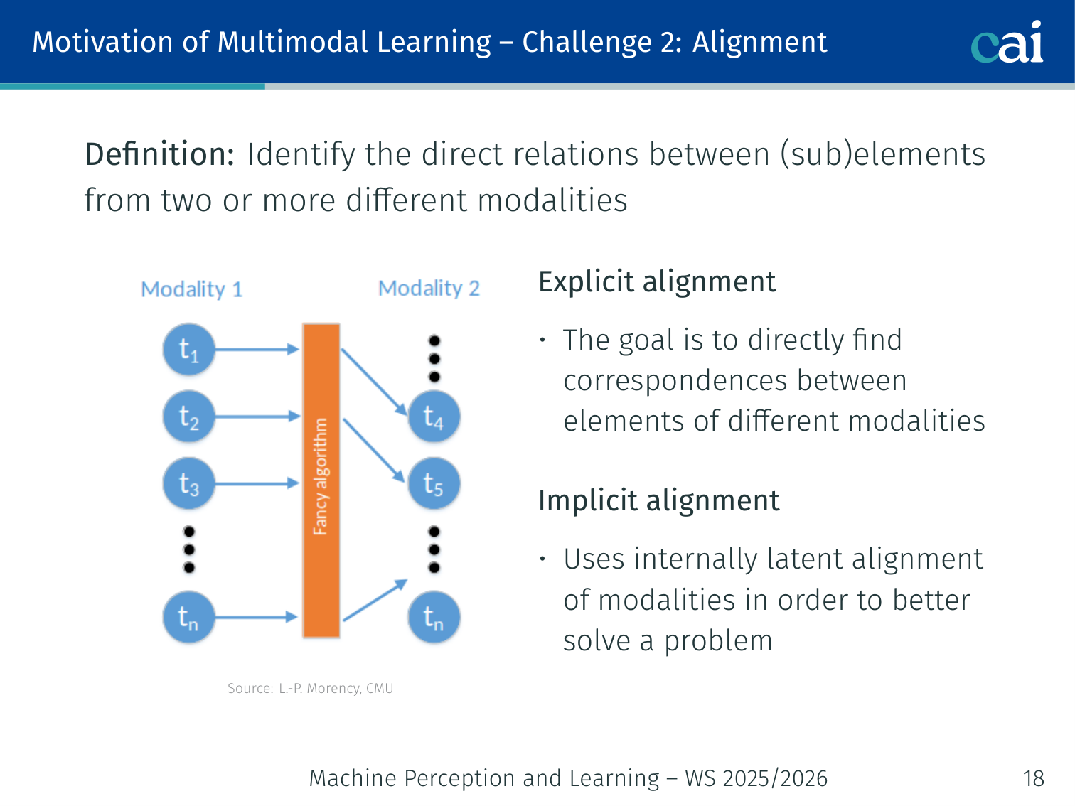
Alignment is about finding which parts of the image match up with which words.

Definition: Identify the direct relations between (sub)elements from two or more different modalities.

Type	Purpose	Example
Explicit alignment	Alignment is the task itself	Match words in a sentence to bounding boxes in an image (Karpathy et al., 2014)
Implicit / Latent alignment	A hidden alignment step that improves a downstream task	Cross-attention in VisualBERT between text tokens and image regions

Use cases for implicit alignment: Machine Translation, Cross-modal retrieval, Image & Video Captioning, VQA, Visual Dialog.

Example: When answering “What colour is the dog’s collar?”, an implicit attention mechanism highlights the word “collar” and the corresponding image region — without any explicit word–region pairing labels in training.

Challenge 3: Translation

Translation is how we map one data type directly to another.

Definition: Change (“translate”) data from one modality to another; the translation relationship is often open-ended or subjective.

Type	Description	Example
Example-based	Retrieve an existing translation from a database	Find the most similar video clip for a caption
Model-driven	A learned model generates the translated output	Neural image captioning, language-guided pose forecasting

Example — Body pose from language: Ahuja & Morency (2019) built Language2Pose, which translates “a person jumps and waves their right arm” into a 3D skeleton pose sequence.

Challenge 4: Fusion

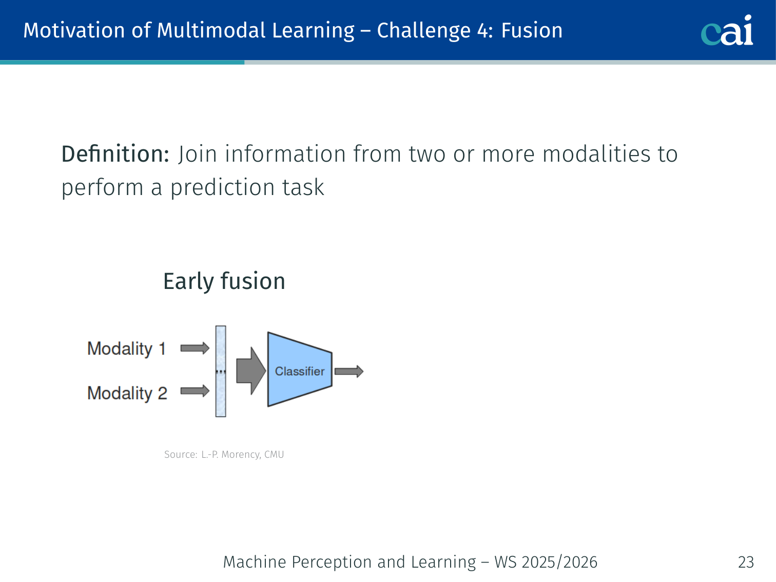
Fusion is where we decide exactly when to mix the different signals.

Definition: Join information from two or more modalities to perform a prediction task.

Strategy	Description	Trade-off
Early fusion	Concatenate raw features from all modalities before any model	Simple; modalities can interfere before useful representations are learned
Late fusion	Process each modality separately; combine predictions (average, voting)	Clean separation; no cross-modal interaction within the model
Model-based / Intermediate	Exchange information at intermediate layers via attention or gating	Highest accuracy; architecturally complex

Model-based techniques include kernel-based methods, graphical models, and deep neural networks with cross-attention.

Tensor Fusion Network (Zadeh et al., 2017)

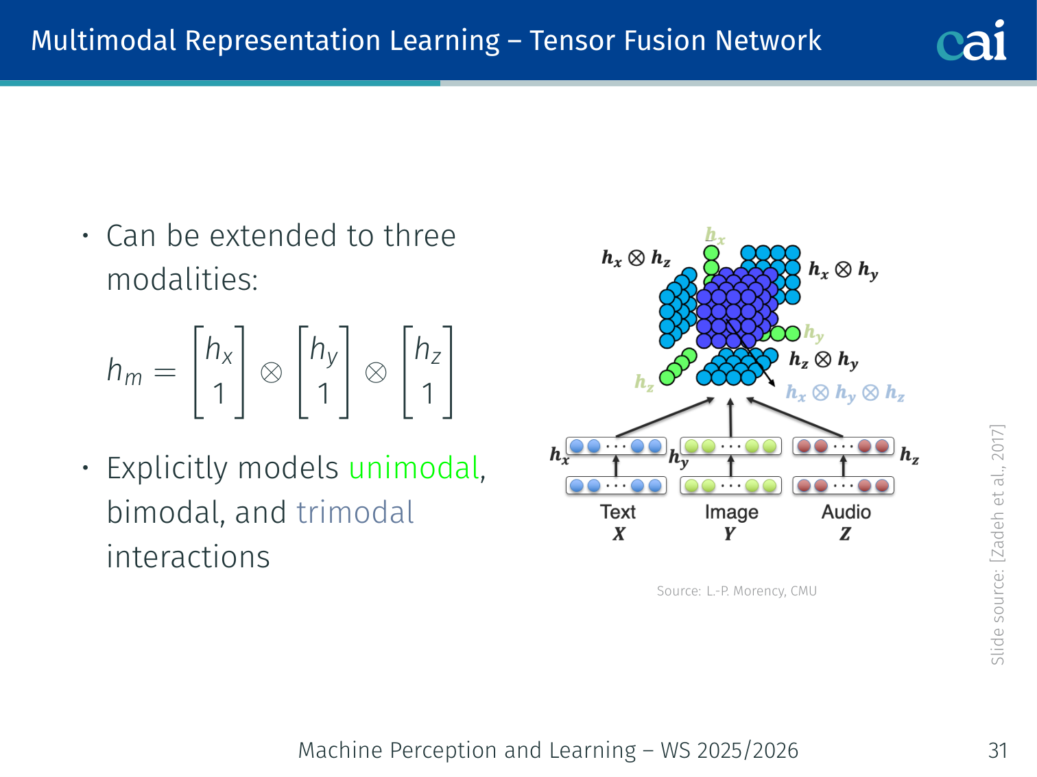
Tensor Fusion picks up on all the interactions between modalities.

Captures unimodal, bimodal, and trimodal interactions via outer products. For two modalities:

$h_{m} = [h_{x} 1] \otimes [h_{y} 1] = h_{x} h_{x} \otimes h_{y} 1 h_{y}$

For three modalities (video, audio, text):

$h_{m} = [h_{x} 1] \otimes [h_{y} 1] \otimes [h_{z} 1]$

Appending $1$ to each unimodal vector means the outer product encodes all subset interactions. Cost is $O (d^{N})$ — expensive for high dimensions.

Example — Sentiment analysis: Three encoders process video frames, audio, and spoken words of a movie review. The tensor fusion layer captures pairwise and triplet interactions before predicting positive/negative sentiment.

Challenge 5: Co-Learning

Co-learning lets us use a data-rich modality to help out a data-poor one.

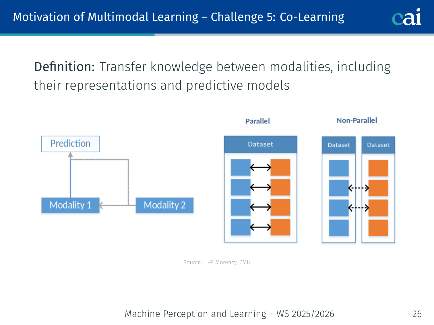
Definition: Transfer knowledge between modalities, including their representations and predictive models.

Useful when one modality has abundant data and another is scarce:

Zero-shot learning: use a rich modality (text) to label examples in a scarce modality (novel visual categories)
Cyclic translation (Pham et al., 2019): learn robust joint representations by cycling language ↔ vision ↔ audio
Weak supervision: use web captions as free image labels

Example: A model trained on English captions can recognise objects in images for categories that have no annotated training images at all (“zero-shot”) — the text description bridges the gap.

3. Multimodal Representation Learning

Joint vs. Coordinated Representations

Joint (fusion)                Coordinated
──────────────────────────    ───────────────────────────
  Image ──┐                  Image ──► Image encoder ──┐
          ├──► Shared space                             ├── cosine constraint
  Text  ──┘                  Text  ──► Text  encoder ──┘
                              (separate spaces, but aligned)

DeViSE — Deep Visual-Semantic Embedding (Frome et al., 2013)

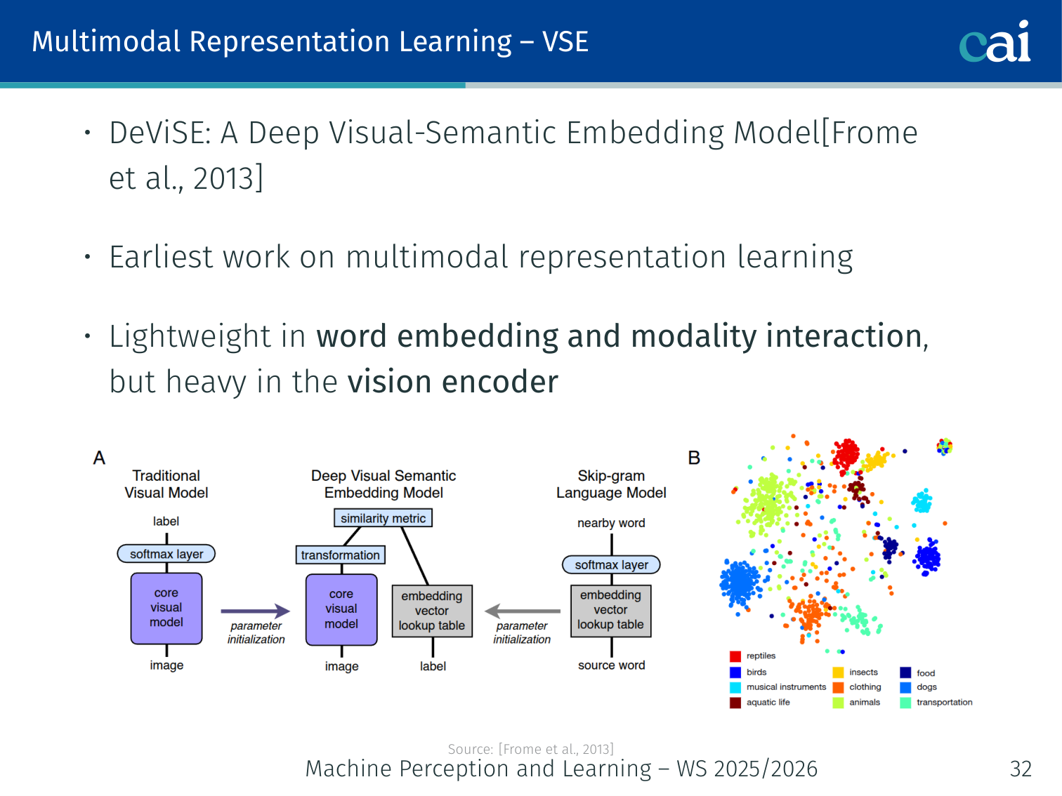
DeViSE maps images into a semantic word-vector space.

The earliest work on multimodal representation learning.

Vision encoder: heavy (ResNet-like CNN)
Word embedding: Word2Vec for class labels
Interaction: lightweight — linear projection + dot product
Train with a ranking loss: correct label should score higher than all incorrect ones

By embedding images into word-vector space, the model gains semantic structure: misclassifying a dog as “cat” is penalised less than “car”, because “cat” and “dog” are close in word-vector space.

Example: At test time DeViSE can recognise unseen classes — if trained on “dog” and “wolf”, it ranks “husky” above “car” for a husky image purely based on word-vector similarity.

CLIP — Contrastive Language-Image Pre-training (Radford et al., 2021)

CLIP uses two encoders to pull matching image-text pairs together.

The landmark multimodal representation model.

💡 Intuition: CLIP as a “Universal Translator”

Think of CLIP not as an image classifier, but as a translator between two languages: Vision and English.

If you show CLIP a picture of a “golden retriever” and the text “golden retriever”, they should both map to the same point in a hidden mathematical space.
Because CLIP was trained on millions of different concepts (not just “cat” and “dog”, but also “a sunset in Paris”, “a broken glass”, “a blueprint of a house”), it has a very rich understanding of the world.

This is why CLIP is the “brain” behind tools like DALL-E and Stable Diffusion — it’s the bridge that tells the generator what a text prompt should actually look like.

🧠 Deep Dive: Contrastive Learning (The Power of “No”)

In standard classification (e.g., ImageNet), the model is only told: “This image is a dog.”

In Contrastive Learning (like CLIP), the model is told two things:

“This image matches this text.” (The Positive)
“And it definitely does NOT match these other 32,000 texts in this batch.” (The Negatives)

Why does this matter? By forcing the model to distinguish between very similar things (e.g., “a photo of a dog” vs. “a photo of a puppy”), we force it to learn much finer details. If we didn’t have negative samples, the model could “cheat” by mapping every image to the same vector, which would give high similarity to every text — but learn absolutely nothing about the world.

Architecture

Image → [Vision Encoder: ViT-B/32 or ResNet] → image embedding (d)
Text  → [Text Encoder: Transformer]           → text  embedding (d)

Both projected to the same d=512 dimensional space.

Component	Weight
Vision encoder	Heavy (large ViT)
Text encoder	Heavy (large Transformer)
Modality interaction	Lightweight (cosine similarity only)

Training Data

400 million (image, text) pairs scraped from the internet — no human annotation. The caption that naturally appears with an image on a webpage is used as weak supervision.

Contrastive Pre-Training Loss

The goal is to make the diagonal of this matrix as large as possible.

Given a batch of $N$ (image, text) pairs, form an $N \times N$ similarity matrix $S$ where $S_{ij} = cosim (i_{i}, t_{j})$ :

$L_{C L I P} = - \frac{1}{2 N} \sum_{i = 1}^{N} [lo g \frac{e ^{S_{ii} / τ}}{\sum _{j} e ^{S_{ij} / τ}} + lo g \frac{e ^{S_{ii} / τ}}{\sum _{j} e ^{S_{ji} / τ}}]$

Diagonal entries $S_{ii}$ are positives (correct image-text pairs); all others are negatives.
$τ$ is a learnable temperature controlling the sharpness of the distribution.
Loss is symmetric: maximises both image→text and text→image retrieval.

Similarity matrix (batch of 4):

            "a dog"  "a cat"  "a car"  "the sky"
dog.jpg   [  0.92     0.18     0.05     0.04  ]
cat.jpg   [  0.17     0.91     0.06     0.03  ]
car.jpg   [  0.04     0.05     0.93     0.03  ]
sky.jpg   [  0.03     0.04     0.05     0.90  ]

The diagonal must be highest in every row and column.

Zero-Shot Classification

After training, CLIP classifies any image without fine-tuning:

Write a text prompt for each class: "a photo of a {class}"
Encode all class prompts → text embeddings
Encode the query image → image embedding
Pick the class with the highest cosine similarity

import clip, torch
from PIL import Image
 
model, preprocess = clip.load("ViT-B/32")
 
image = preprocess(Image.open("dog.jpg")).unsqueeze(0)
texts = clip.tokenize(["a photo of a dog", "a photo of a cat", "a photo of a car"])
 
with torch.no_grad():
    img_feat = model.encode_image(image)
    txt_feat  = model.encode_text(texts)
 
img_feat /= img_feat.norm(dim=-1, keepdim=True)
txt_feat  /= txt_feat.norm(dim=-1, keepdim=True)
probs = (100.0 * img_feat @ txt_feat.T).softmax(dim=-1)
 
print(probs)  # tensor([[0.91, 0.07, 0.02]]) → "dog" wins

CLIP achieves 76.2% zero-shot top-1 on ImageNet, matching supervised ResNet-50 without seeing any ImageNet training images.

Key Properties

Property	Detail
Prompt engineering matters	`"a photo of a {class}"` outperforms bare class name
Robust features	Generalises well to distribution shifts (texture, style, domain)
Zero-shot capable	No task-specific fine-tuning needed
Open vocabulary	Any concept expressible in text can be a class

Embedding Space Arithmetic

"a red car"  ≈  image(red car)
"a blue car" ≈  image(blue car)

image(red car) − image(car) + text("boat") ≈ image(red boat)

CLIP Variants

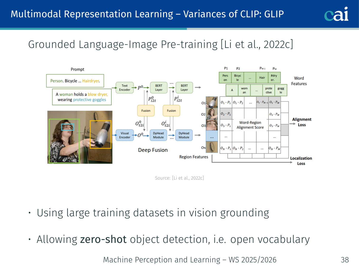
GLIP — Grounded Language-Image Pre-training (Li et al., 2022)

GLIP extends CLIP's ideas down to individual object bounding boxes.

Extends CLIP to object detection: instead of image-level contrastive loss, GLIP aligns language phrases with bounding boxes
Enables zero-shot object detection (open vocabulary)
Uses large-scale grounding datasets (COCO, Visual Genome, + web data)

Example: Given the prompt “the red fire hydrant”, GLIP draws a bounding box around it — no task-specific detector training needed.

LSeg — Language-Driven Semantic Segmentation (Li et al., 2022)

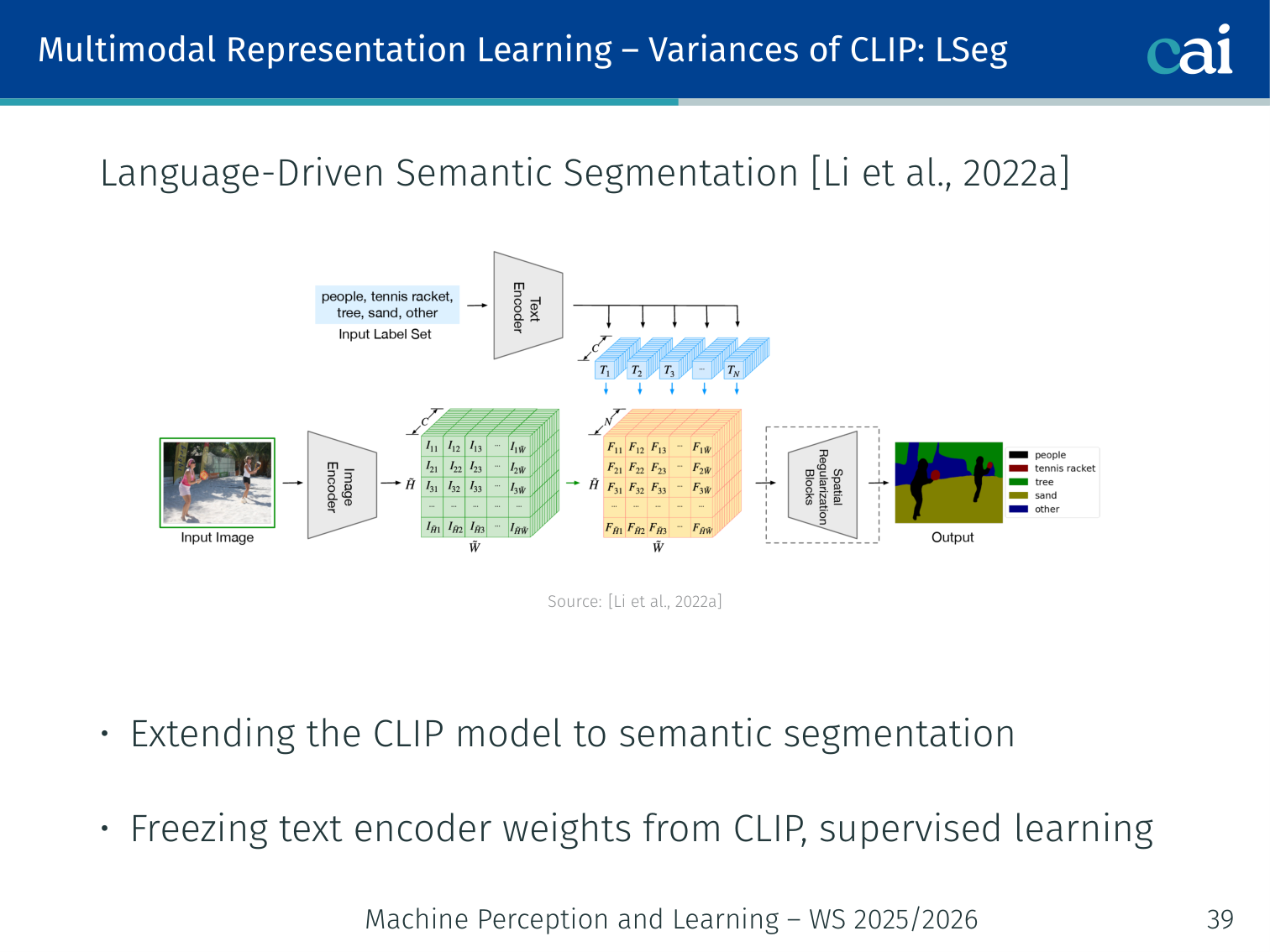
LSeg takes it even further by aligning text labels with individual pixels.

Extends CLIP to pixel-level semantic segmentation
Freezes the CLIP text encoder; supervises the image encoder + decoder to produce segmentation maps aligned with text embeddings
Each pixel is classified by its distance to text embeddings of category names

Example: LSeg can segment any category described in text — even categories not seen during supervised training — because the frozen text encoder provides open-vocabulary embeddings.

4. Multimodal Alignment

Motivation

We need alignment to know exactly what the model is looking at.

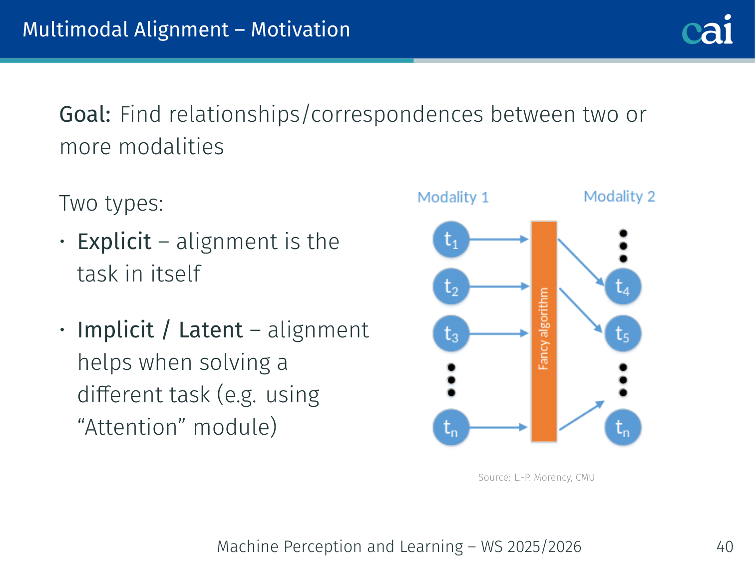
Goal: Find relationships/correspondences between elements of two or more modalities.

Alignment Type	Purpose	Example
Explicit	Alignment is the end task	Match words in a caption to image regions
Implicit / Latent	Internal alignment improves a downstream task	Cross-attention in VQA

Cross-modal transformers let one modality 'look' at another via attention.

The queries come from one modality while keys and values come from the other.

In standard self-attention, $Q$ , $K$ , $V$ all come from the same sequence. In a cross-modal attention module, the query comes from one modality and the key/value from another:

$CrossAttn (Q_{A}, K_{B}, V_{B}) = softmax (\frac{Q _{A} K _{B}^{⊤}}{d _{k}}) V_{B}$

This allows modality A to selectively read information from modality B.

Example: For VQA, text question tokens form queries $Q_{text}$ ; image patch embeddings form $K_{img}, V_{img}$ . Cross-attention tells each word which image regions are most relevant to it.

Case Study: VisualBERT (Li et al., 2019)

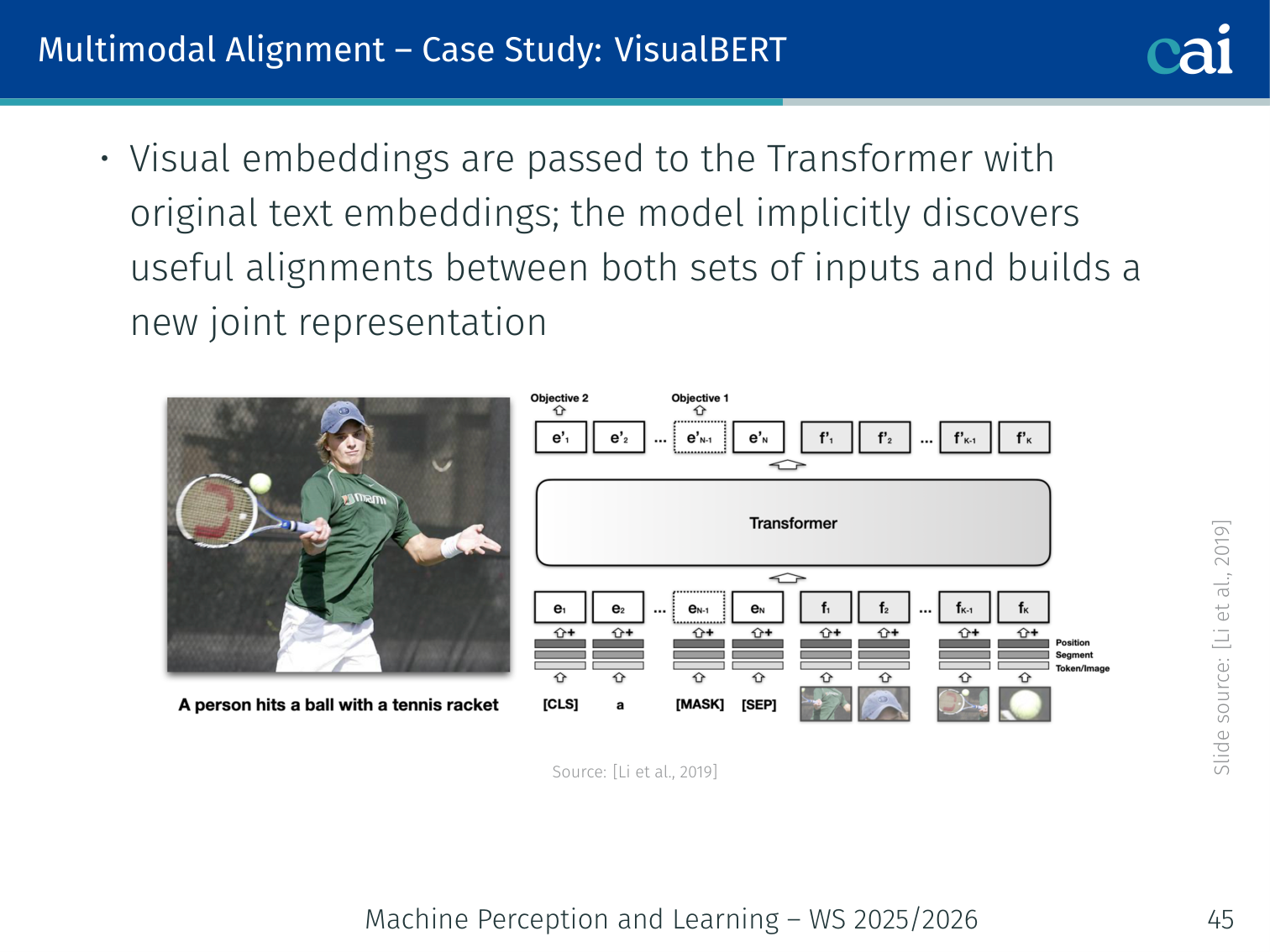
VisualBERT just throws everything into one big transformer stream.

Concatenate text tokens (BERT tokeniser) and visual embeddings (one per bounding region from Faster R-CNN), then feed jointly to a standard BERT Transformer
Self-attention can attend across modalities — the model implicitly discovers useful alignments

Visual embedding $f$ for one bounding region:

$f = f_{o} + f_{s} + f_{p}$

Component	Role
$f_{o}$	Visual feature of the bounding region (CNN output)
$f_{s}$	Segment embedding (“this is an image token, not text”)
$f_{p}$	Positional embedding (aligns words and image regions spatially)

Example — NLVR2: Given an image and “There is exactly one dog left of the red cube”, VisualBERT attends over regions labelled “dog” and “cube” to verify the spatial claim.

Case Study: ViLBERT (Lu et al., 2019)

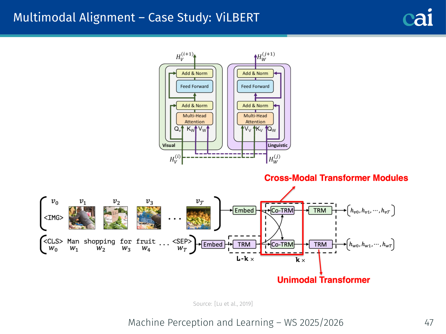
ViLBERT keeps two streams but lets them talk via co-attention.

Two-stream architecture: separate Transformer for image and text, connected via co-attention layers
Co-attention: image tokens attend to all text tokens; text tokens attend to all image tokens — simultaneously
More flexible than VisualBERT’s single stream; better at fine-grained cross-modal tasks

	VisualBERT	ViLBERT
Streams	Single	Dual
Alignment	Implicit (joint self-attention)	Explicit co-attention layers

Case Study: HowTo100M + MIL-NCE (Miech et al., 2019/2020)

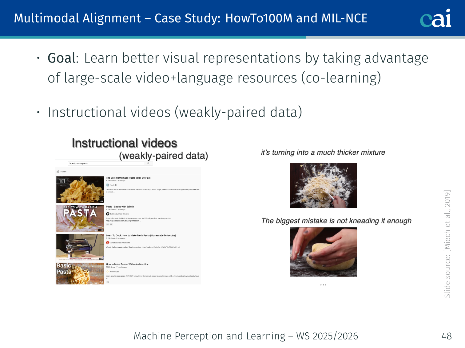
MIL-NCE helps the model learn even when captions aren't perfectly timed.

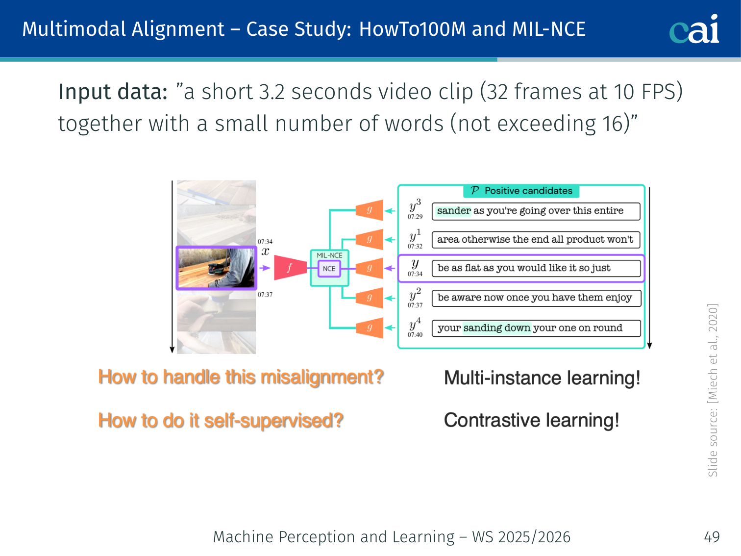
Instead of one exact match, we treat a window of captions as potential positives.

HowTo100M: 100M instructional video clips from YouTube with ASR-generated subtitles
Captions are weakly aligned — the subtitle at second $t$ may describe something at $t - 5$

MIL-NCE (Multiple Instance Learning Noise Contrastive Estimation) handles noisy alignment. Given video $x$ , positive subtitle set $P_{i}$ , and negative set $N_{i}$ :

$L = - lo g \frac{\sum _{y^{+} \in P_{i}} e x p ( s ( x , y ^{+} ))}{\sum _{y^{+} \in P_{i}} e x p ( s ( x , y ^{+} )) + \sum _{y^{-} \in N_{i}} e x p ( s ( x , y ^{-} ))}$

Each clip’s subtitle set is treated as a bag of positives — at least one subtitle should match the video, even if not all do.

Input: 3.2-second video clip (32 frames at 10 FPS) + up to 16 subtitle words.

Example: A cooking clip shows someone whisking eggs. The subtitle “and now you want to beat the eggs vigorously” arrives a few seconds early. MIL-NCE treats all nearby subtitle segments as potential positives, reducing the penalty for off-by-a-few-seconds noise.

Case Study: ViLT — Vision-and-Language Transformer (Kim et al., 2021)

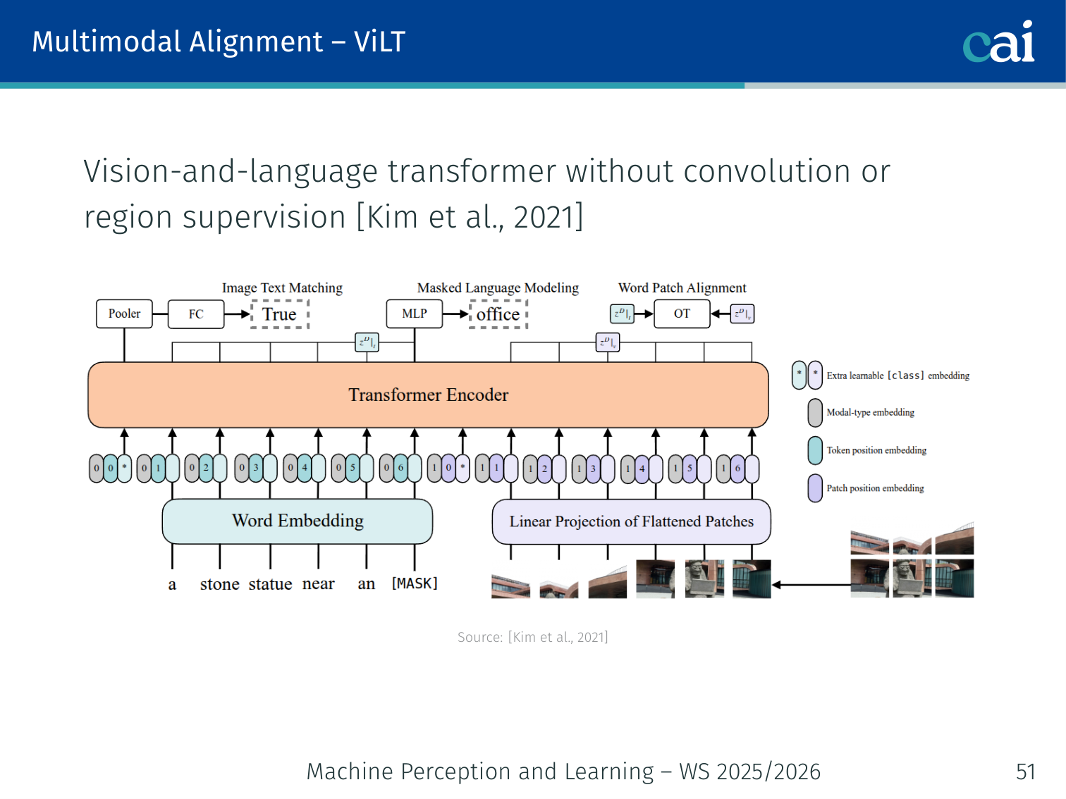
ViLT skips the heavy object detector and just uses raw image patches.

No region features, no object detectors. Uses raw patch embeddings (ViT-style) + text token embeddings, fed jointly into one Transformer
60× faster than VisualBERT at inference (no Faster R-CNN bottleneck)
Training losses: Masked Language Modelling (MLM) + Image Text Matching (ITM)

Model	Vision encoder	Interaction	Speed
DeViSE	Heavy CNN	Lightweight	Fast
VisualBERT	Detector (heavy)	Moderate	Slow
ViLT	Patch embed (light)	Heavy (full Transformer)	Fast
CLIP	Heavy ViT	Lightweight	Fast

ALBEF — Align Before Fuse (Li et al., 2021)

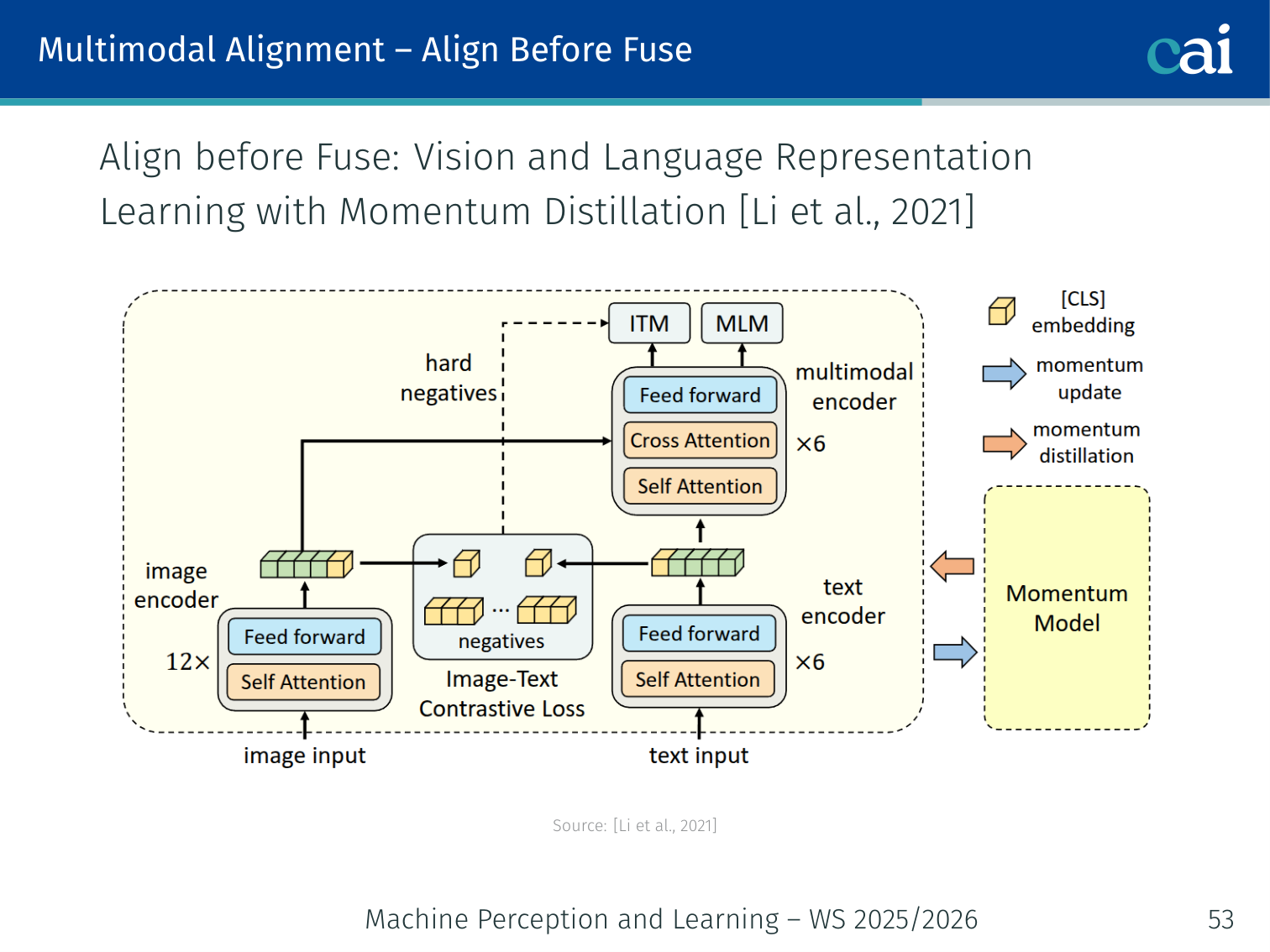
ALBEF makes sure features are aligned before it tries to fuse them.

Key insight: explicitly align image and text embeddings before fusing them — so the fusion module gets clean aligned inputs rather than having to align and fuse simultaneously.

Integrates MoCo (He et al., 2020) momentum encoder + ViT + BERT.

Loss Components

It uses three different losses to get the alignment and fusion right.

Loss	Purpose
Image-Text Contrastive (ITC)	Align image and text unimodal embeddings (CLIP-style)
Image-Text Matching (ITM)	Binary: does this (image, text) pair match?
Masked Language Modelling (MLM)	Predict masked text tokens using image context

Hard negative mining: for ITM, use the negative pair with the highest ITC similarity (not a random negative) — forces the model to learn fine-grained distinctions.

Example: For a batch of beach images and ocean captions, a random negative is easy to reject (e.g., a caption about mountains). The hard negative is a different beach caption — very similar but not the correct pair — forcing the model to learn subtle cross-modal differences.

BLIP — Bootstrapping Language-Image Pre-training (Li et al., 2022)

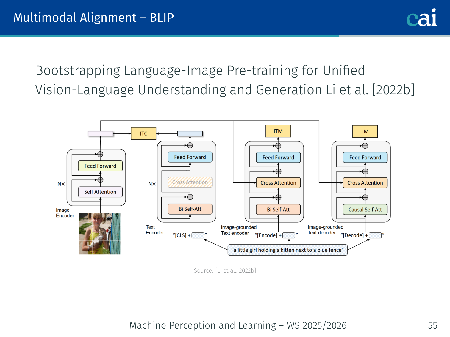
BLIP cleans up messy web data by filtering and generating its own captions.

An improved version of ALBEF with two innovations:

Unified encoder+decoder: handles both understanding (retrieval, classification) and generation (captioning) with shared weights
CapFilt (Caption + Filter): bootstrapping to improve data quality:
- Captioner generates synthetic captions for noisy web images
- Filter removes captions (original or generated) that do not match the image
- Result: higher-quality dataset than raw web data

Example — CapFilt in action: A web image shows a sunset, but the scraped alt-text says “click here for more sunsets”. The Filter removes this useless caption. The Captioner generates “a vibrant orange sunset over calm ocean waters”, which passes the Filter. The model trains on the better caption.

5. Multimodal Reasoning

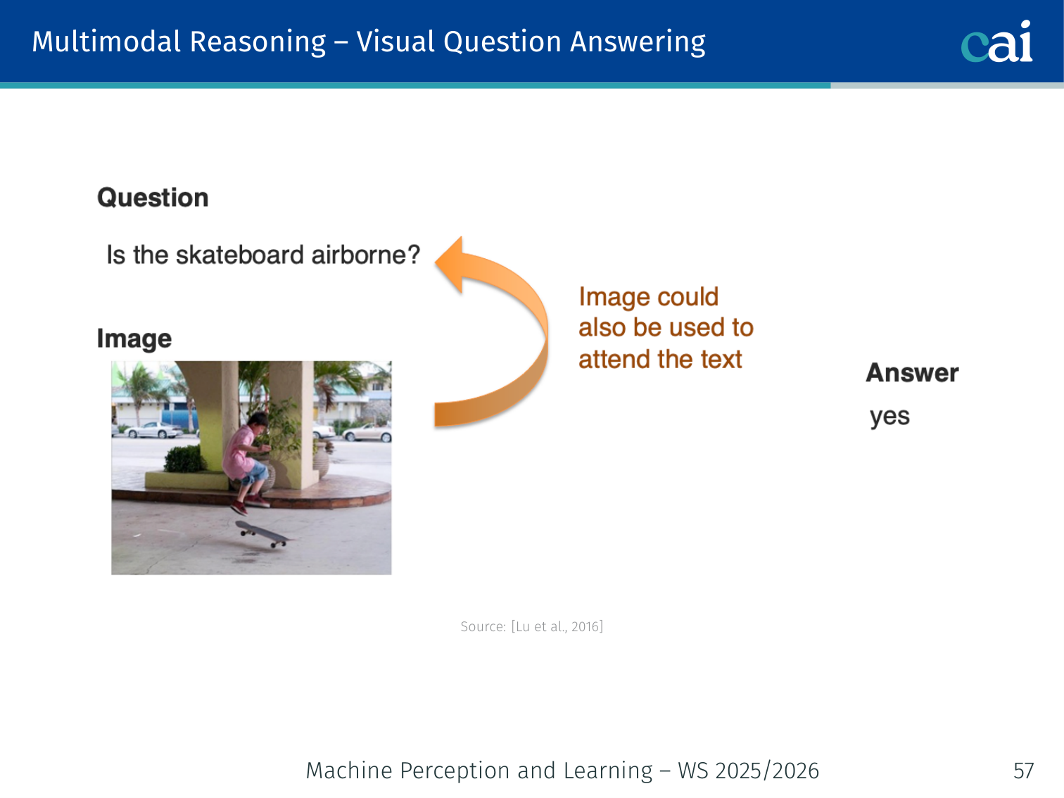
Visual Question Answering (VQA)

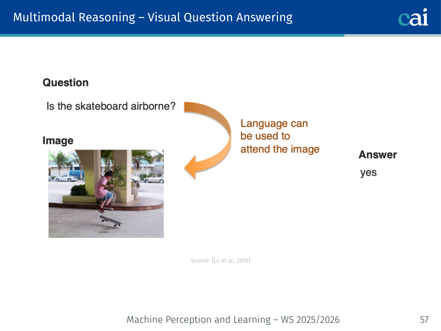
Introduction to Visual Question Answering (VQA) tasks and examples

Comparing different types of questions in the VQA dataset

Task: Given an image and a natural language question, produce a natural language answer.

Examples of increasing difficulty:

“What colour is the car?” → “Red” (perception)

“How many chairs are around the table?” → “4” (counting)

“Is the traffic light showing red or green?” → “Green” (fine-grained)

“What would happen if the person on the left steps forward?” → commonsense + spatial reasoning

Hierarchical Co-Attention (Lu et al., 2016)

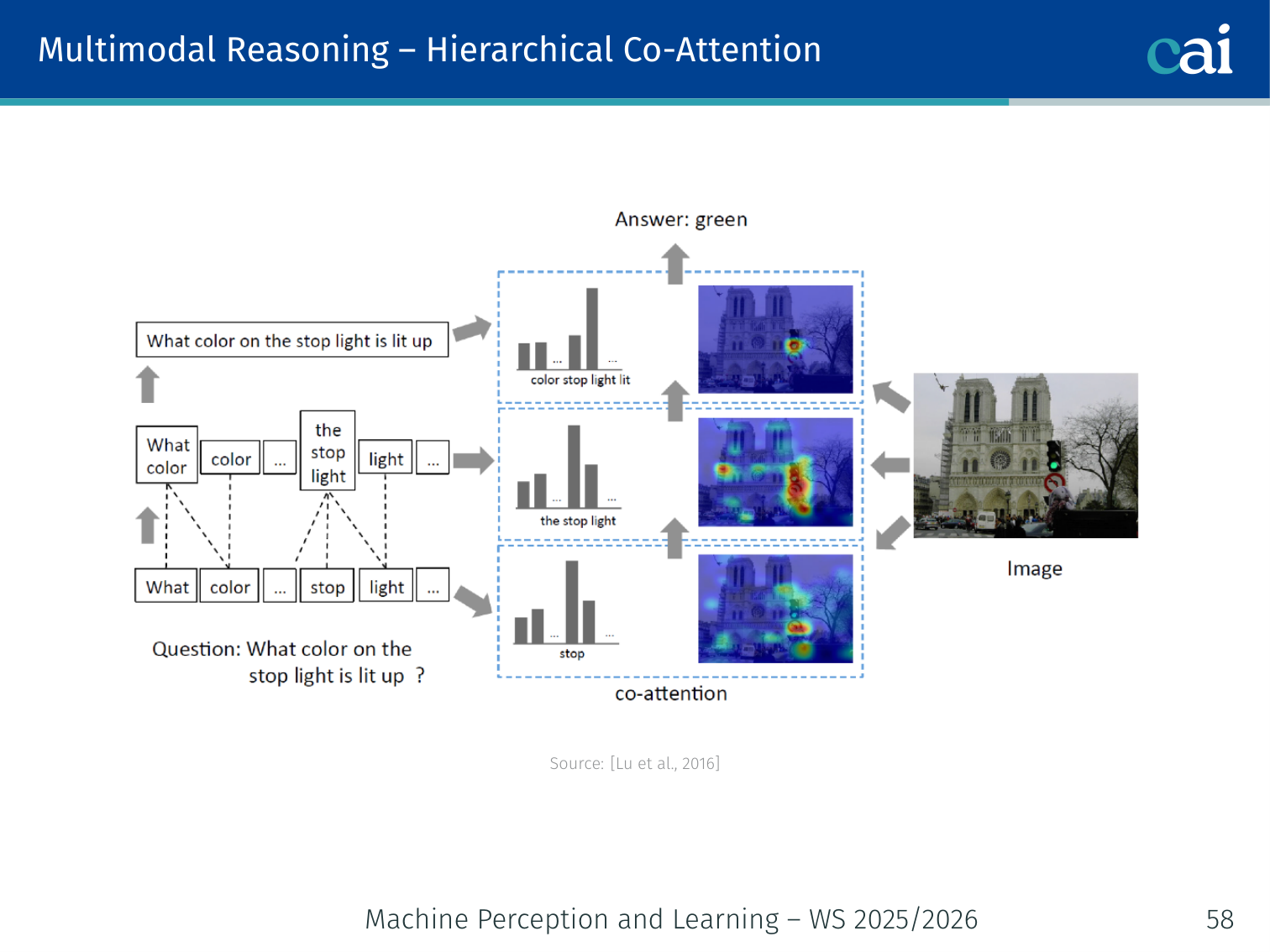
Architecture of Hierarchical Co-Attention for VQA across words, phrases, and sentences

Two parallel attention streams, each conditioned on the other:

Question encodings ──► Q-guided Image Attention  ──► attended image v̂
Image encodings    ──► V-guided Question Attention ──► attended question q̂

[v̂ ; q̂] ──► prediction head

Computed at three levels of granularity:

Word level: individual question words ↔ image patches
Phrase level: multi-word phrases ↔ spatial regions
Sentence level: full question ↔ global image

Example: For “What colour is the large sphere to the left of the metallic cube?”, word-level attention highlights “large”, “sphere”, “left”, “metallic cube”. Phrase-level groups these into an object reference. Sentence-level selects the colour attribute.

Stacked Attention Networks (Yang et al., 2016)

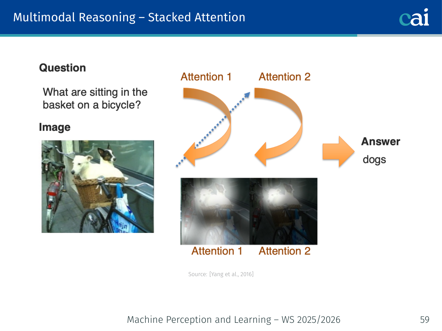
Architecture of Stacked Attention Networks using multi-hop refinement

Use multiple hops of attention — each hop refines image attention based on the partial answer from the previous hop:

Hop 1: Q + V → attention α₁ → attended image v̂₁
Hop 2: Q + v̂₁ → refined attention α₂ → v̂₂
...
Final: Q + v̂_K → answer prediction

Example: For “What is to the right of the red cube?”, Hop 1 attends broadly to red objects. Hop 2 uses that result to attend specifically to what is spatially to the right. The final answer is predicted from the refined feature.

Other Attention-Based Models

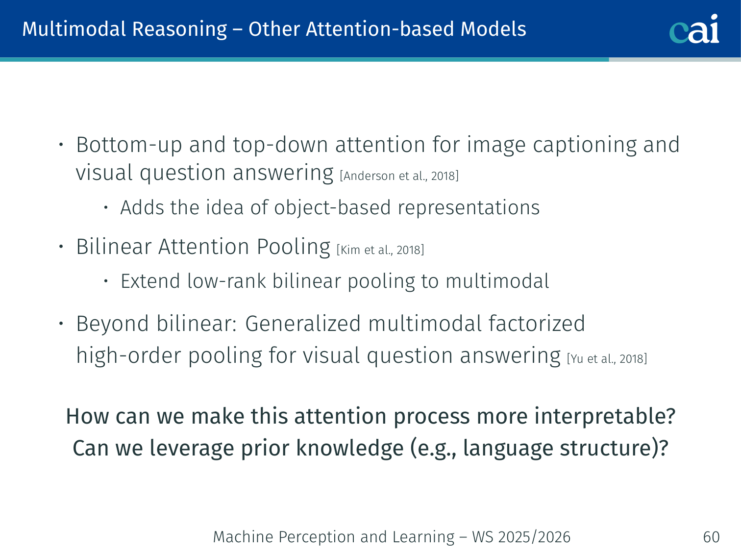
Comparison of different attention-based models for VQA and captioning

Model	Key Idea
Bottom-up and top-down attention (Anderson et al., 2018)	Object-level representations from Faster R-CNN; top-down question-conditioned attention over detected objects
Bilinear Attention Pooling (Kim et al., 2018)	Low-rank bilinear pooling between image and text — efficient pairwise interaction
Generalized High-Order Pooling (Yu et al., 2018)	Extends bilinear to higher-order interactions for richer fusion

Open research questions: how to make attention more interpretable? Can we leverage explicit language structure (syntax trees, dependency graphs)?

Neural Module Networks — V1 (Andreas et al., 2015)

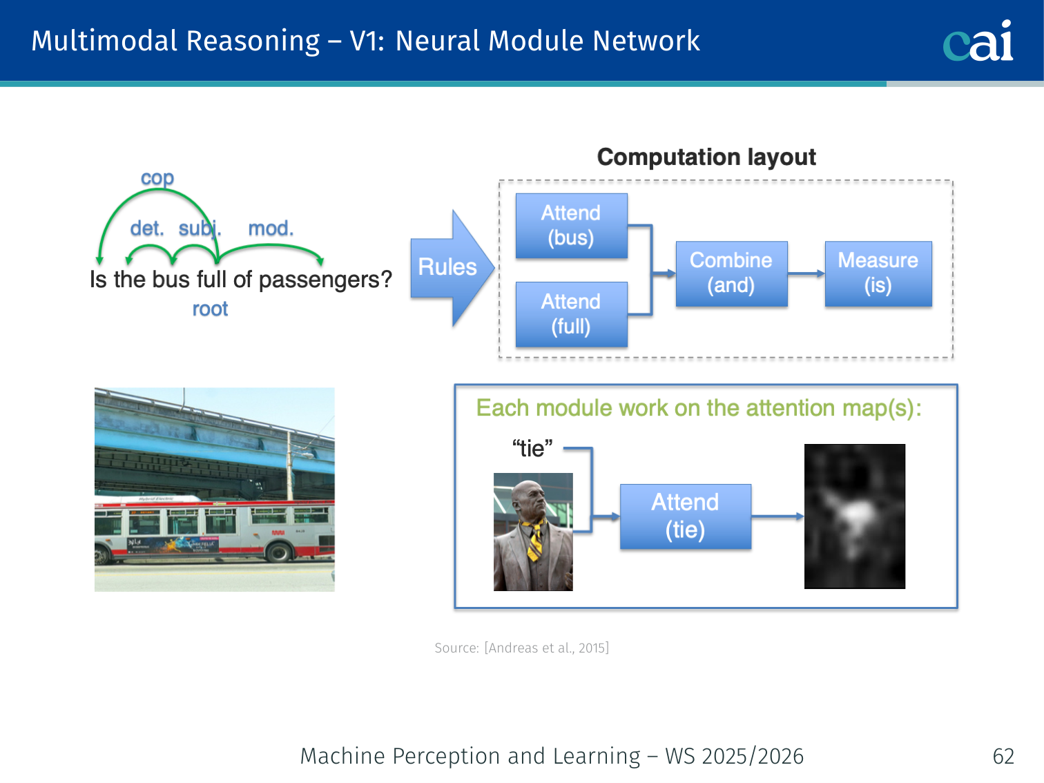
Architecture of Neural Module Networks (V1) using a rule-based parser

Key insight: decompose the question into a program (a composition of neural modules), then execute it over the image.

Parse the question → a layout (directed tree of operations)
Assemble predefined neural modules according to the layout
Execute the assembled network on the image

Example modules:

find[dog] — produces an attention map highlighting dogs
relate[left-of] — shifts attention spatially
describe[colour] — predicts the colour of the attended region
count — counts distinct attended objects
and, or — logical compositions

Example: Question “What colour is the ball to the left of the blue cube?”

Program: describe[colour]( relate[left-of]( find[blue-cube], find[ball] ) )

Each module runs sequentially; the final output is the colour class.

Limitation: requires a separate (rule-based) parser to generate the module layout.

CLEVR — A Dataset for Visual Reasoning (Johnson et al., 2017)

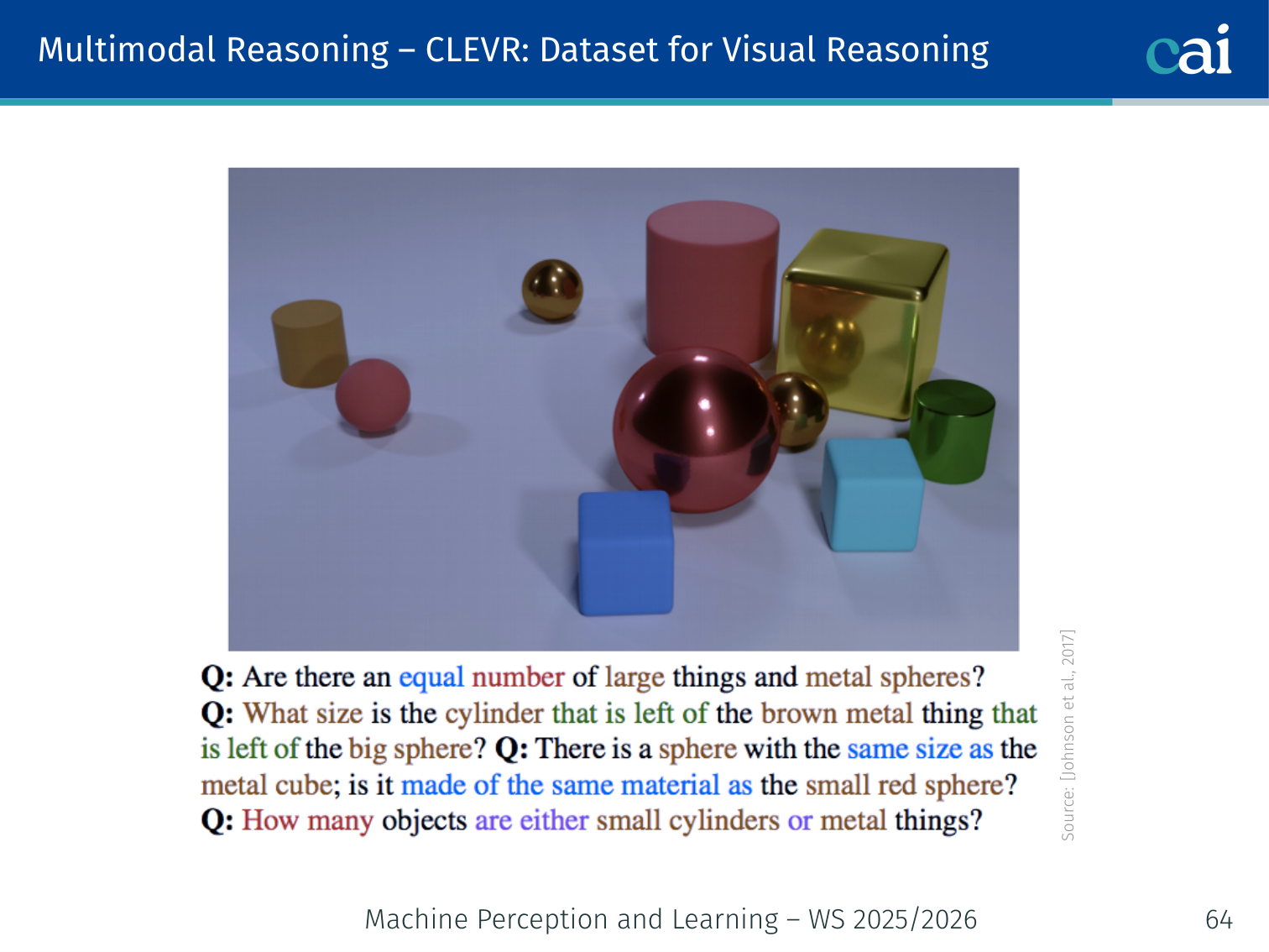
Examples from the CLEVR dataset for compositional visual reasoning

A synthetic benchmark for compositional visual reasoning:

3D-rendered scenes of simple objects (cubes, spheres, cylinders) in various colours, sizes, materials
Questions generated programmatically from scene graphs → guaranteed ground truth programs
Designed so that statistical shortcuts fail — models must reason compositionally

Example questions:

“Is there a large red sphere made of rubber?” “How many silver metallic objects are the same size as the yellow cube?” “What colour is the object to the left of the large metal sphere behind the blue rubber cylinder?”

Neural Module Networks — V2: End-to-End Learning (Hu et al., 2017)

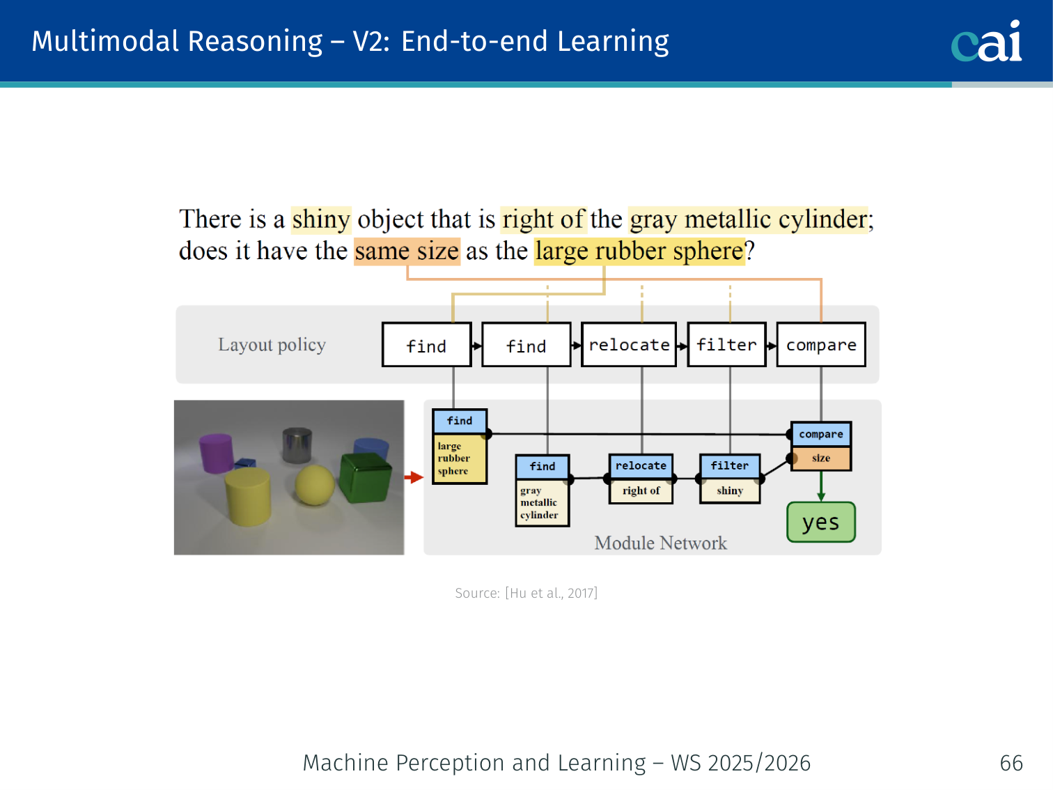
Architecture of Neural Module Networks (V2) with end-to-end program generation

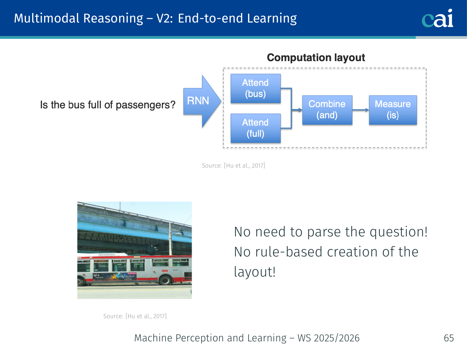
Visualizing the program generator and executor in end-to-end NMNs

Removes the rule-based parser from V1:

A program generator (seq2seq network) takes the question and predicts the layout automatically without explicit parse supervision
A program executor assembles and runs the modules
The whole system is trained jointly end-to-end

Question ──► Program Generator ──► Layout Tree
                                       │
Image    ──────────────────────────────▼
                               Module Assembly + Execution
                                       │
                                       ▼
                               Answer prediction

Example: “How many red things are left of the large sphere?” is fed to the program generator, which proposes count(filter[red](relate[left-of](find[large-sphere]))) — without explicit parse annotation. The executor runs this on the image and returns a count.

PyTorch Implementation: Prototypical Networks (Few-Shot)

import torch
import torch.nn as nn
import torch.nn.functional as F
 
class ProtoNet(nn.Module):
    def __init__(self, encoder):
        super().__init__()
        # The encoder is typically a CNN that maps images to a feature vector
        self.encoder = encoder
 
    def forward(self, support_images, query_images, n_way, n_support):
        """
        Args:
            support_images: labeled examples (n_way * n_support, C, H, W)
            query_images: unlabeled examples to classify (n_query, C, H, W)
            n_way: number of classes in the current task
            n_support: number of examples per class (the 'k' in k-shot)
        """
        # 1. Get embeddings for both support and query sets
        # Concatenate them to run the encoder only once for efficiency
        x = torch.cat([support_images, query_images], 0)
        z = self.encoder(x) # (Total_images, Feature_dim)
        z_dim = z.size(-1)
 
        # 2. Extract prototypes
        # Reshape support embeddings to (n_way, n_support, Feature_dim)
        z_support = z[:n_way*n_support].view(n_way, n_support, z_dim)
        # Compute the mean vector for each class -> this is the PROTOTYPE
        prototypes = z_support.mean(1) # Result: (n_way, Feature_dim)
 
        # 3. Classify Query Images
        z_query = z[n_way*n_support:] # Embeddings of the images we want to label
        # Compute Squared Euclidean distance from every query to every prototype
        # dists[i, j] is distance from query 'i' to prototype 'j'
        dists = torch.cdist(z_query, prototypes, p=2)**2
 
        # 4. Return log-probabilities
        # We use negative distance because closer = more probable
        return F.log_softmax(-dists, dim=1)

Key Few-Shot Concepts:

n-way, k-shot: A task where you must choose between n classes, and you only have k labeled examples per class to learn from.
The Prototype: The central assumption is that there exists a single representative point for each class in the embedding space.
Metric Learning: Unlike standard classifiers, the model isn’t learning a fixed decision boundary; it’s learning an embedding space where similar things are close together.

Summary

Representation Learning Models

Comparison table of representation learning models: DeViSE, CLIP, GLIP, and LSeg

Model	Vision encoder	Text encoder	Interaction	Key contribution
DeViSE (2013)	Heavy CNN	Word2Vec	Dot product	Earliest visual-semantic embedding; semantic label space
CLIP (2021)	Heavy ViT	Heavy Transformer	Cosine sim	Contrastive pre-training at scale; zero-shot
GLIP (2022)	Detector	Transformer	Grounded boxes	Zero-shot object detection
LSeg (2022)	ViT + decoder	Frozen CLIP text	Pixel–text alignment	Open-vocabulary segmentation

Alignment Models

Model	Architecture	Key Innovation
VisualBERT (2019)	Single-stream	Region features + text → joint self-attention
ViLBERT (2019)	Dual-stream	Co-attention layers between modalities
HowTo100M + MIL-NCE (2019/20)	Video + text	MIL loss handles temporal noise in ASR captions
ViLT (2021)	Single-stream patches	No region detectors; 60× faster
ALBEF (2021)	Dual encoder + fusion	ITC aligns before ITM fuses; hard negative mining
BLIP (2022)	Unified enc.+dec.	CapFilt bootstrapping; generation + understanding

Reasoning Models

Model	Key Idea
Hierarchical co-attention (Lu 2016)	Parallel V↔Q attention at word/phrase/sentence levels
Stacked Attention (Yang 2016)	Multi-hop refinement of image attention guided by partial answer
Bottom-up + top-down (Anderson 2018)	Object-level attention; question-conditioned top-down guidance
NMN V1 (Andreas 2015)	Program decomposition into interpretable neural modules
CLEVR (Johnson 2017)	Compositional reasoning benchmark; no statistical shortcuts
NMN V2 / E2E (Hu 2017)	End-to-end learned program generation; no parser required

References

Baltrušaitis, Ahuja & Morency (2018). Multimodal machine learning: A survey and taxonomy. IEEE TPAMI.
Frome et al. (2013). DeViSE: A deep visual-semantic embedding model. NeurIPS.
Radford et al. (2021). Learning transferable visual models from natural language supervision. ICML. (CLIP)
Li et al. (2022a). Language-driven semantic segmentation. arXiv. (LSeg)
Li et al. (2022c). Grounded language-image pre-training. CVPR. (GLIP)
Zadeh et al. (2017). Tensor Fusion Network for Multimodal Sentiment Analysis. EMNLP.
Kiros et al. (2014). Unifying visual-semantic embeddings with multimodal neural language models. arXiv.
Tsai et al. (2019). Multimodal Transformer for Unaligned Multimodal Language Sequences. ACL.
Li et al. (2019). VisualBERT: A simple and performant baseline for vision and language. arXiv.
Lu et al. (2019). ViLBERT: Pretraining task-agnostic visiolinguistic representations. NeurIPS.
Miech et al. (2019). HowTo100M: Learning a text-video embedding by watching 100M narrated clips. ICCV.
Miech et al. (2020). End-to-end learning of visual representations from uncurated instructional videos. CVPR.
Kim et al. (2021). ViLT: Vision-and-language transformer without convolution or region supervision. ICML.
Li et al. (2021). Align before fuse: Vision and language representation learning with momentum distillation. NeurIPS. (ALBEF)
Li et al. (2022b). BLIP: Bootstrapping language-image pre-training. ICML.
Lu et al. (2016). Hierarchical question-image co-attention for VQA. NeurIPS.
Yang et al. (2016). Stacked Attention Networks for Image Question Answering. CVPR.
Anderson et al. (2018). Bottom-up and top-down attention for image captioning and VQA. CVPR.
Kim et al. (2018). Bilinear Attention Networks. NeurIPS.
Andreas et al. (2015). Deep compositional question answering with neural module networks. arXiv.
Johnson et al. (2017). CLEVR: A diagnostic dataset for compositional language and visual reasoning. CVPR.
Hu et al. (2017). Learning to reason: End-to-end module networks for VQA. ICCV.
Ahuja & Morency (2019). Language2Pose: Natural language grounded pose forecasting. 3DV.
Ngiam et al. (2011). Multimodal deep learning. ICML.
Srivastava & Salakhutdinov (2012). Multimodal learning with deep Boltzmann machines. NeurIPS.
Pham et al. (2019). Found in translation: Learning robust joint representations by cyclic translations between modalities. AAAI.

Applied Exam Focus

CLIP: Uses Contrastive Learning to align images and text in a shared latent space. The goal is to maximize the cosine similarity of matching pairs.
Zero-Shot Transfer: Because CLIP learns concepts (e.g., “a photo of a dog”) rather than fixed labels, it can classify objects it was never explicitly trained on.
Modality Gap: Despite alignment, image and text features often occupy distinct clusters in the latent space, which is an ongoing research challenge.

Previous: L06 — ViT | Back to MPL Index | Next: (y-08) IML | (y) Return to Notes | (y) Return to Home

Yusuf's Thoughts

Explorer