L08 — Interactive Machine Learning (IML)

Previous: L07 — Multimodal | Back to MPL Index | Next: (y-09) VAE

Mental Model First

• Interactive ML starts from one practical fact: human attention is expensive, so we should spend it where it teaches the model the most.
• Active learning is not about labeling more data; it is about labeling the right data.
• Most of the lecture is really about query strategy: uncertainty, diversity, disagreement, and how to avoid biasing yourself with bad sample selection.
• If one question guides this lecture, let it be: when should a model ask for help, and which example is worth asking about next?

Introduction

💡 Intuition: Active Learning as “Smart Questioning”

Imagine a student studying for an exam.

• Passive Learning: The student reads the entire 500-page textbook from cover to cover. It’s thorough, but very slow, and they might spend hours reading things they already know.
• Active Learning (iML): The student skim-reads the textbook, identifies the 10 most confusing problems, and asks the teacher (the Oracle) to explain only those 10.

By asking the “right” questions, the student learns much faster and with much less effort from the teacher. In ML, this teacher is the human expert, and their time is the most expensive resource we have.

---

🧠 Deep Dive: The Labeling Bottleneck

Why do we need iML at all?

1. Cost: Labeling a single medical scan might take a radiologist 10 minutes and cost €50. We cannot afford to label 100,000 of them.
2. Expertise: You can’t just hire someone on MTurk to label a Higgs-Boson particle track in a physics experiment. You need a physicist.
3. Dynamic Data: If you are building a fraud detector, the “rules” of fraud change every day. You need to constantly update the model with new, relevant examples.

Interactive ML is the bridge that makes it possible to build high-quality models in these “data-starved” or “expert-heavy” domains.

---

Automatic vs. Interactive ML

Traditional ML vs. Interactive ML—here's where the human comes in.

Most ML today is automatic machine learning (aML): algorithms that interact with agents and optimize their learning without human involvement during training. This works great when you have large, clean, labeled datasets.

This “big data + end-to-end automation” paradigm powers many successful applications, including recommender systems, autonomous vehicles, and industrial AI systems. The lecture’s framing point is that these successes depend heavily on abundant data and well-specified objectives; they do not automatically transfer to every domain.

But sometimes you still need a human in the loop:

• Small or multiple datasets — not enough data for aML to be reliable
• Rare events — how do you get enough examples of a 1-in-10,000 failure?
• NP-hard problems — subspace clustering, protein folding, k-anonymisation, graph colouring

Definition

A formal look at iML: putting the human right in the learning loop.

Interactive Machine Learning (iML) := algorithms that interact with agents (which can be humans) and that can optimise their learning behaviour through this interaction. — Holzinger, 2015

The human is seen as an agent involved in the actual learning phase, influencing years such as distance or cost functions step by step — not just checking results at the end.

This matters especially in health informatics and other high-stakes settings, where decision making can be viewed as a search problem in a very large hypothesis space under tight time constraints. A “good” decision is not only about raw prediction accuracy; it is about expected utility under domain-specific costs, risks, and failure modes.

Types of ML on a Spectrum

The ML spectrum, ranging from totally unsupervised to fully interactive.

Type	Labels	Human Role
Unsupervised	None	Check results at end
Supervised	All data labeled	Provide labels & features upfront
Semi-supervised	Some labeled, rest unlabeled	Label a small seed set
Interactive (iML)	Adaptive	Inform/correct the model during learning

Who Can Be “In the Loop”?

The different agents we can have in the loop, from experts to the crowd.

• A single expert (e.g. a radiologist annotating cancer scans)
• A crowd (e.g. Amazon Mechanical Turk workers)
• Multiple heterogeneous agents (domain experts + crowd + automated tools)
• Nature-inspired agents (evolutionary algorithms, etc.)

Limits of Pure aML and of Human Interaction

The lecture also highlights two complementary cautions:

• Pure aML struggles when data are scarce, rare events matter, or the search problem is combinatorial / NP-hard
• Human-in-the-loop systems introduce their own issues: robustness of human feedback, subjectivity, transferability across tasks, and open questions around evaluation and reproducibility

---

Motivating Applications

Example 1: k-Anonymisation of Medical Data

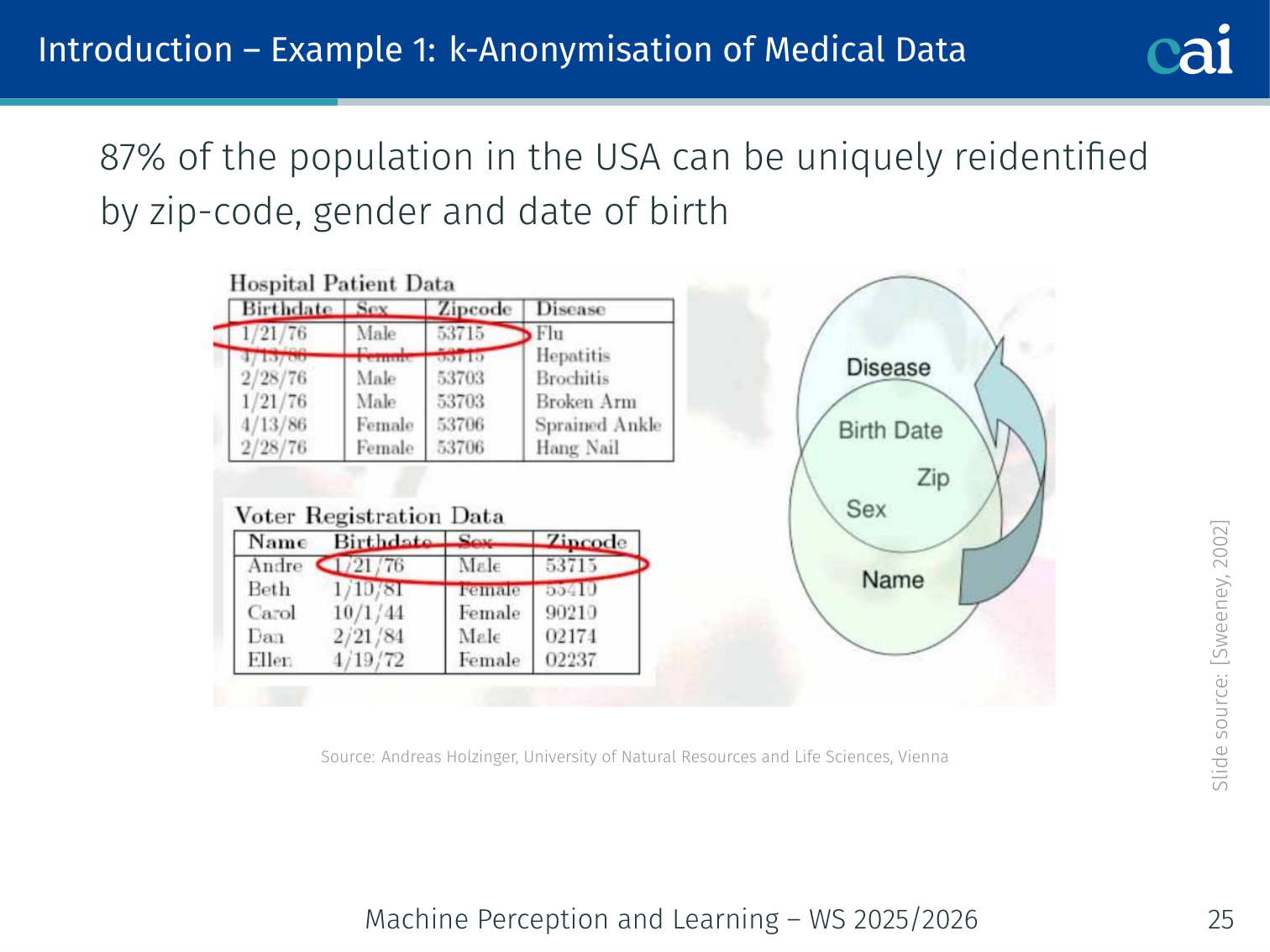
Using iML to help with k-anonymization for sensitive medical data.

87% of the US population can be uniquely re-identified by zip-code, gender, and date of birth (Sweeney, 2002). k-Anonymity requires transforming data so each record is indistinguishable from at least k−1 others. Finding the optimal transformation is NP-hard — a human expert can guide the search interactively.

Example 2: Protein Folding

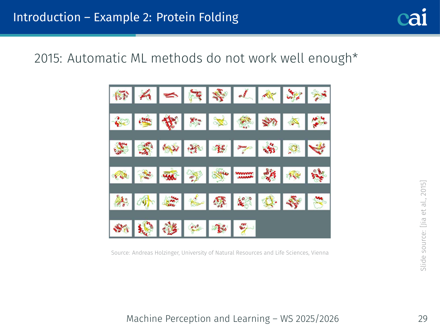
How human guidance can help tackle the complex protein folding problem.

Proteins are the building blocks of life; their 3D structure is determined by their amino acid sequence. Predicting that structure from sequence is an old, extremely hard problem. As of 2015, automatic ML methods did not work well enough. A human-in-the-loop could guide structure search.

Recent breakthrough: AlphaFold (DeepMind, Jumper et al., 2021) achieved remarkable accuracy using deep learning, largely removing the need for human guidance — showing that when data is sufficient, aML can eventually surpass iML.

Example 3: Subspace Clustering

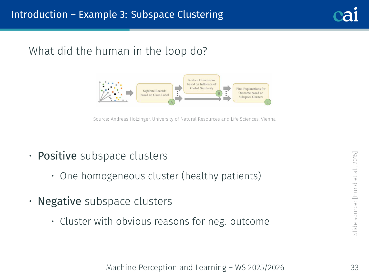
Spotting positive and negative clusters in subspace clustering.

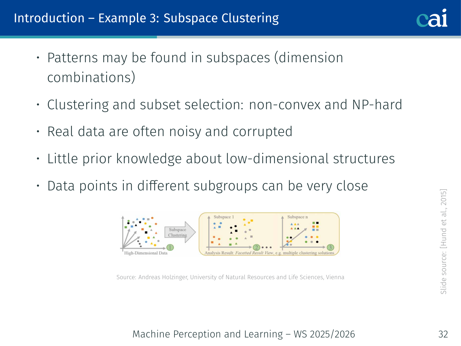
Patterns in high-dimensional data often hide within these subspaces.

Patterns in high-dimensional data often live in subsets of dimensions (subspaces). Clustering in subspaces is non-convex and NP-hard, data is often noisy, and there’s little prior knowledge about the low-dimensional structure. Human experts can:

• Identify positive subspace clusters (e.g. one homogeneous cluster of healthy patients)
• Identify negative clusters with obvious reasons for poor outcomes

---

Semi-supervised Learning

Setup

Given:

• $S_l=(x_1,y_1),(x_2,y_2),\dots ,(x_m,y_m)$ — labeled examples drawn i.i.d. from distribution $D$, with $y_i=c^{\ast }(x_i)$
• $S_u=x_1,\dots ,x_{m_u}$ — unlabeled examples drawn i.i.d. from $D$

Goal: find a classifier with small generalization error ${\text{err}}_D(h)=P(h(x)\ne c^{\ast }(x))$

Key Insight

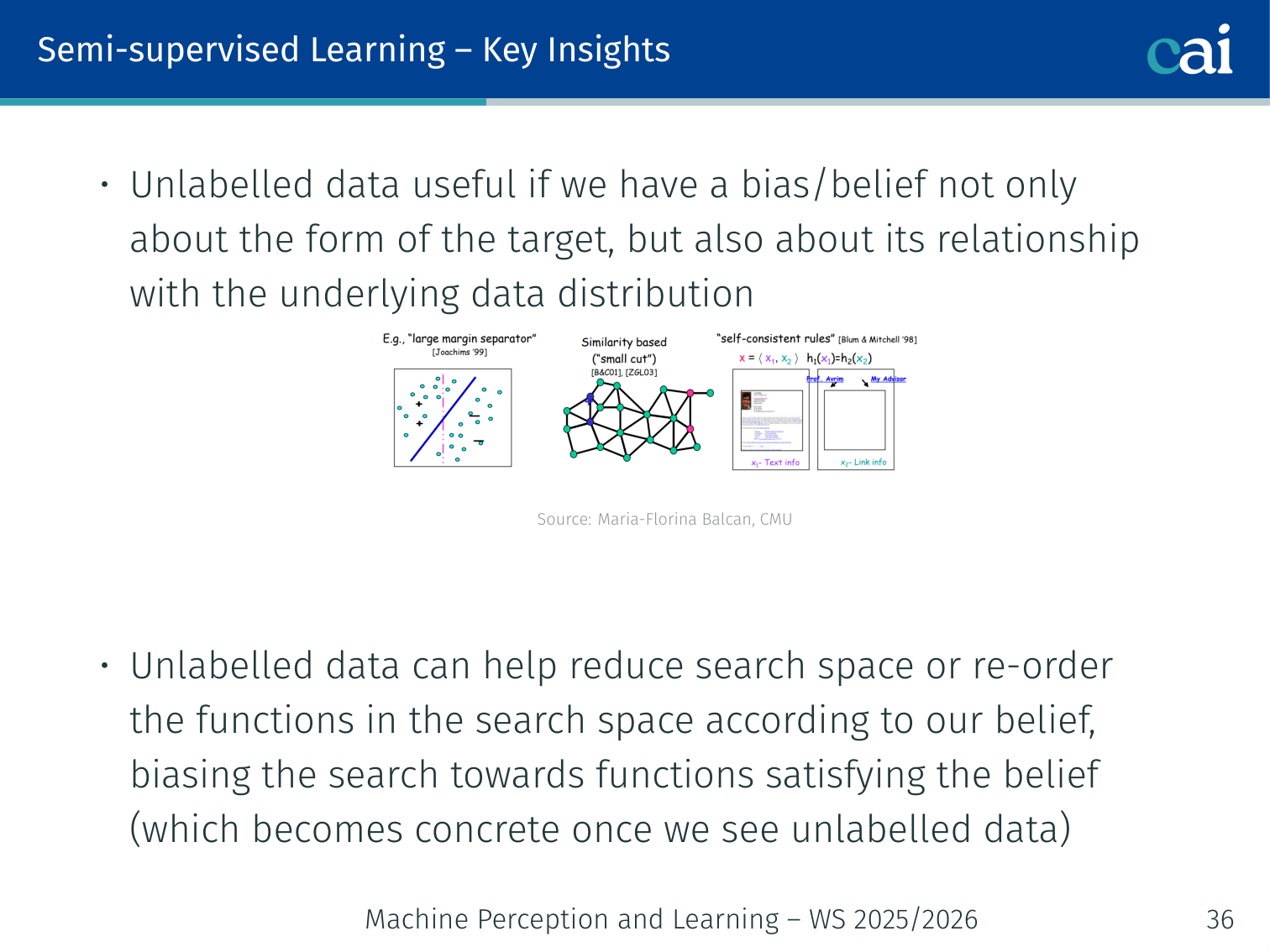
Unlabeled data helps by shrinking the search space and biasing our function.

Unlabeled data is useful only if we have a belief not just about the form of the target function, but also about its relationship with the underlying data distribution.

Unlabeled data can:

• Reduce the search space
• Re-order functions in the search space according to our belief
• Bias the search toward functions consistent with the data manifold

(Zhu and Goldberg, 2009)

Fundamental Questions (General Discriminative Model)

The big questions for discriminative models when dealing with unlabeled data.

• How much unlabeled data is needed? — depends on complexity of $H$ and the compatibility notion
• Can unlabeled data reduce the number of labeled examples needed?
• Is the target function compatible with the data distribution? — helpfulness depends on this

Example: Two concentric rings of data points (inner ring = class A, outer ring = class B). With only labeled data you might draw the wrong boundary; with unlabeled data you can “see” the ring structure and place the boundary between the rings.

---

Active Learning

Batch vs. Selective Sampling (Stream)

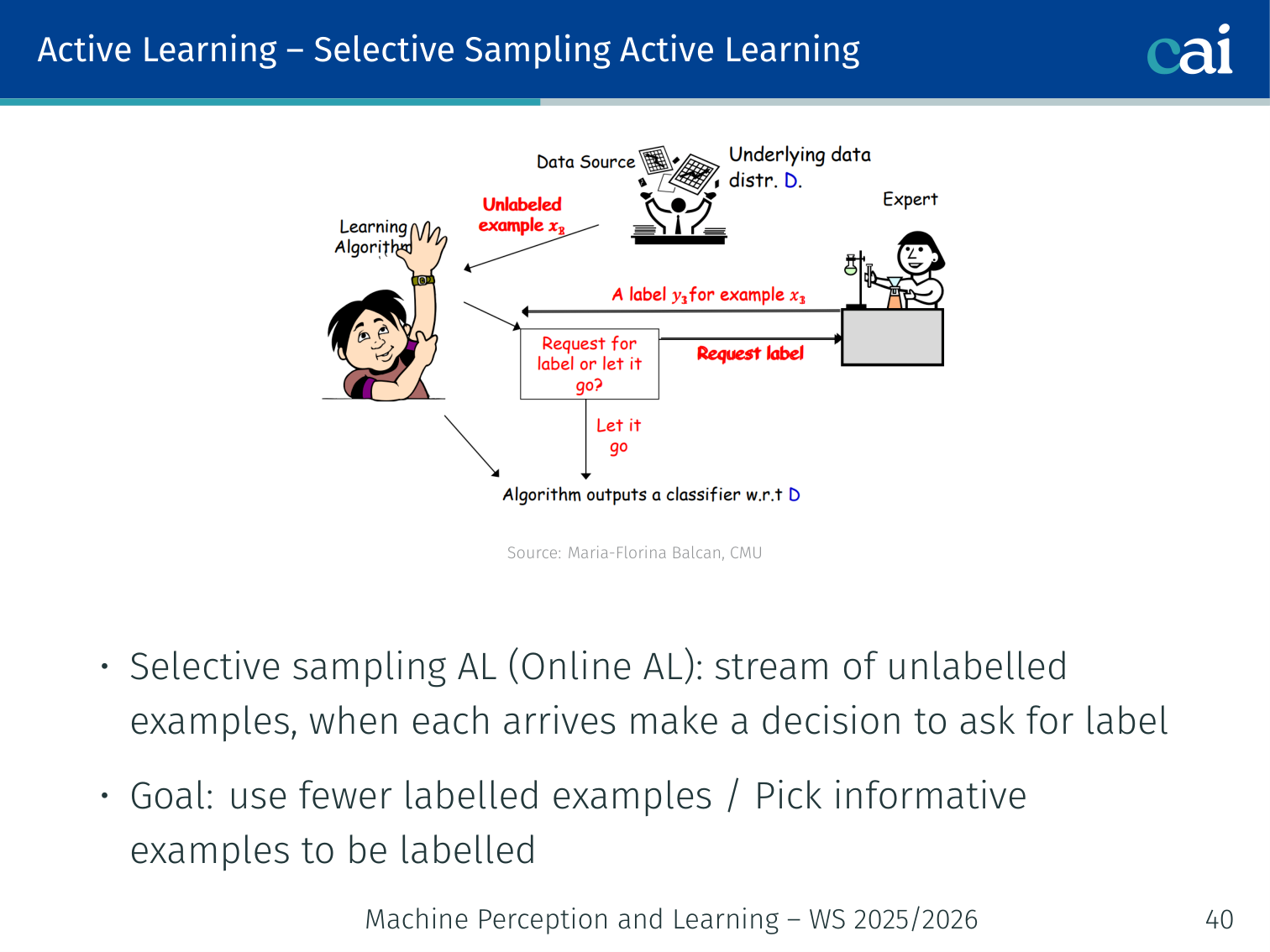
Batch Active Learning vs. Selective Sampling in a live data stream.

Mode	Description
Batch Active Learning	Learner picks specific examples from a pool to label
Selective Sampling (Online AL)	A stream of unlabeled examples arrives; learner decides on-the-fly whether to query

In both cases the goal is to use far fewer labeled examples than passive (random) learning by picking informative examples.

Can Adaptive Querying Actually Help?

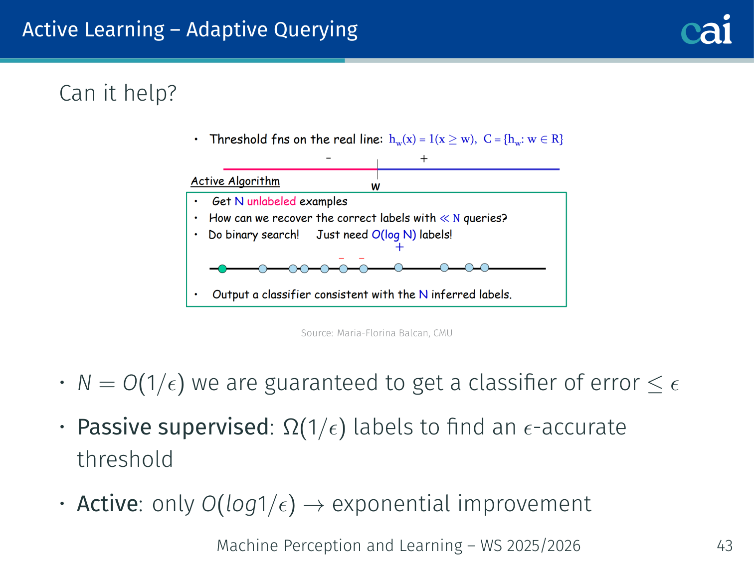
Comparing label complexity: active learning is like doing a binary search.

Yes — exponentially so (sometimes).

Consider learning a threshold classifier on the real line:

• Passive supervised: need $\Omega (1/\epsilon )$ labels to find an $\epsilon$-accurate threshold
• Active learning: only $O(\log 1/\epsilon )$ labels needed — an exponential improvement

Binary search is the perfect analogy:

Range: [0, 1]    True threshold: 0.73

Query midpoint 0.5  → label is +  (threshold > 0.5)
Query midpoint 0.75 → label is -  (threshold < 0.75)
Query midpoint 0.625 → label is + (threshold > 0.625)
...

After k queries: threshold known to within 1/2^k — log(1/ε) queries suffice.
Passive learning needs 1/ε queries to get the same ε accuracy.

In practice: Observed on Newsgroups (20K documents) and CIFAR-10 (60K images) — active learning reaches the same accuracy with far fewer labels (Jain et al., 2010).

---

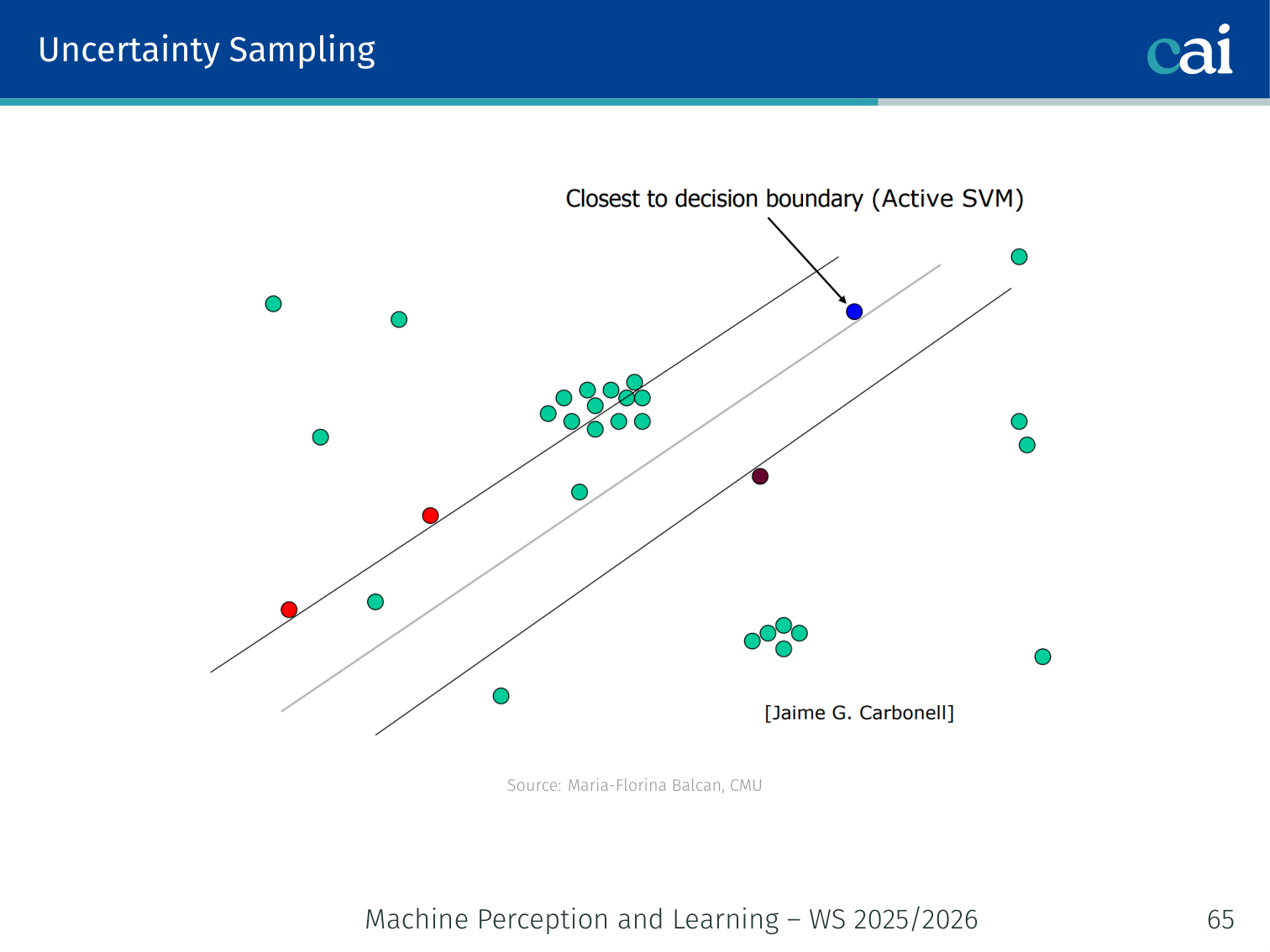
Active SVM — Uncertainty Sampling in Practice

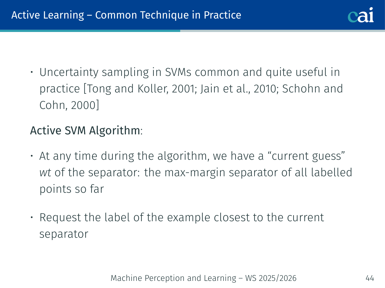
Active SVM in action: we query the points right on the decision boundary.

A common and effective technique (Tong & Koller, 2001; Schohn & Cohn, 2000):

Algorithm:

1. Maintain the current max-margin separator $w_t$ over all labeled points so far
2. At each step, request the label of the example closest to the decision boundary (smallest margin = most uncertain)
3. Retrain the SVM and update $w_t$

from sklearn.svm import SVC
import numpy as np
 
model = SVC(kernel='rbf')
labeled_idx = np.random.choice(len(X_pool), size=10)  # seed
 
for _ in range(num_rounds):
    model.fit(X_pool[labeled_idx], y[labeled_idx])
 
    distances = np.abs(model.decision_function(X_pool))
    distances[labeled_idx] = np.inf  # exclude already labeled
 
    query_idx = np.argmin(distances)   # closest to boundary → most uncertain
    labeled_idx = np.append(labeled_idx, query_idx)
    # oracle labels X_pool[query_idx] ...

⚠️ Sampling Bias Warning

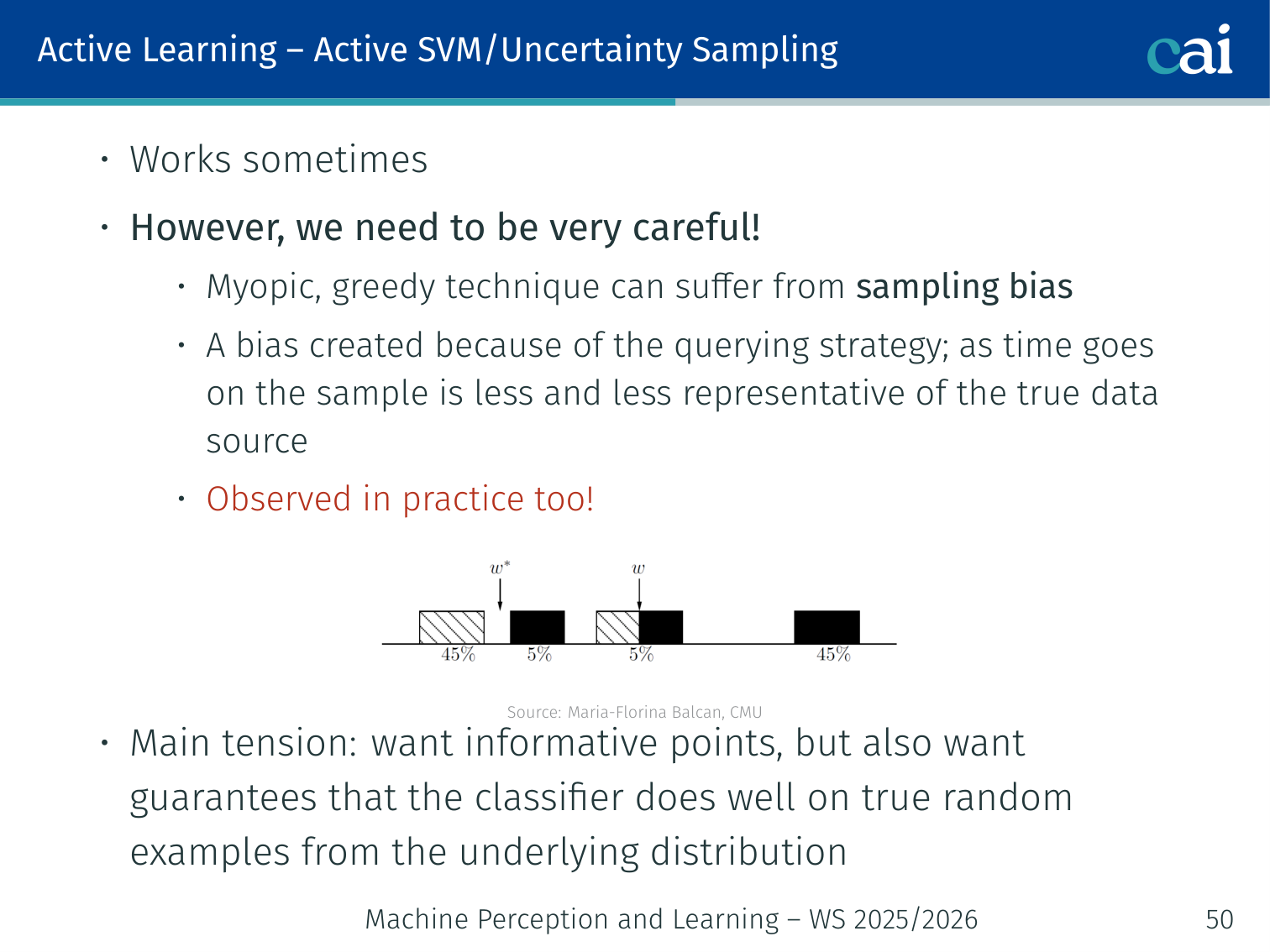
The risk of sampling bias when we're too greedy with uncertainty sampling.

Uncertainty sampling is myopic and greedy. Over time the queried sample becomes less representative of the true data distribution — the model excels near the boundary but may fail elsewhere. (Dasgupta, 2011)

Main tension: we want informative points (near boundary) and guarantees that the classifier performs well on truly random examples from the underlying distribution.

---

Version Spaces

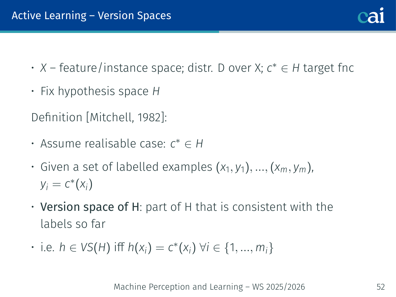
The Version Space, bounded by our most general and most specific hypotheses.

Definition (Mitchell, 1982):

• $X$ — feature/instance space; distribution $D$ over $X$; target $c^{\ast }\in H$
• Realisable case: $c^{\ast }\in H$
• Version space $VS(H)$: the part of $H$ consistent with all labels so far

$h\in VS(H)⟺h(x_i)=c^{\ast }(x_i)\forall i$

The version space is bounded by:

• GB — maximally general positive hypothesis boundary (outer boundary)
• SB — maximally specific positive hypothesis boundary (inner boundary)

Example: Data on a circle in ${\mathbb{R}}^2$; $H$ = homogeneous linear separators. After 3 positive and 3 negative labels placed on the circle, only separators that correctly divide those 6 points remain in the version space. Each new label eliminates more separators, shrinking the version space.

---

Region of Disagreement

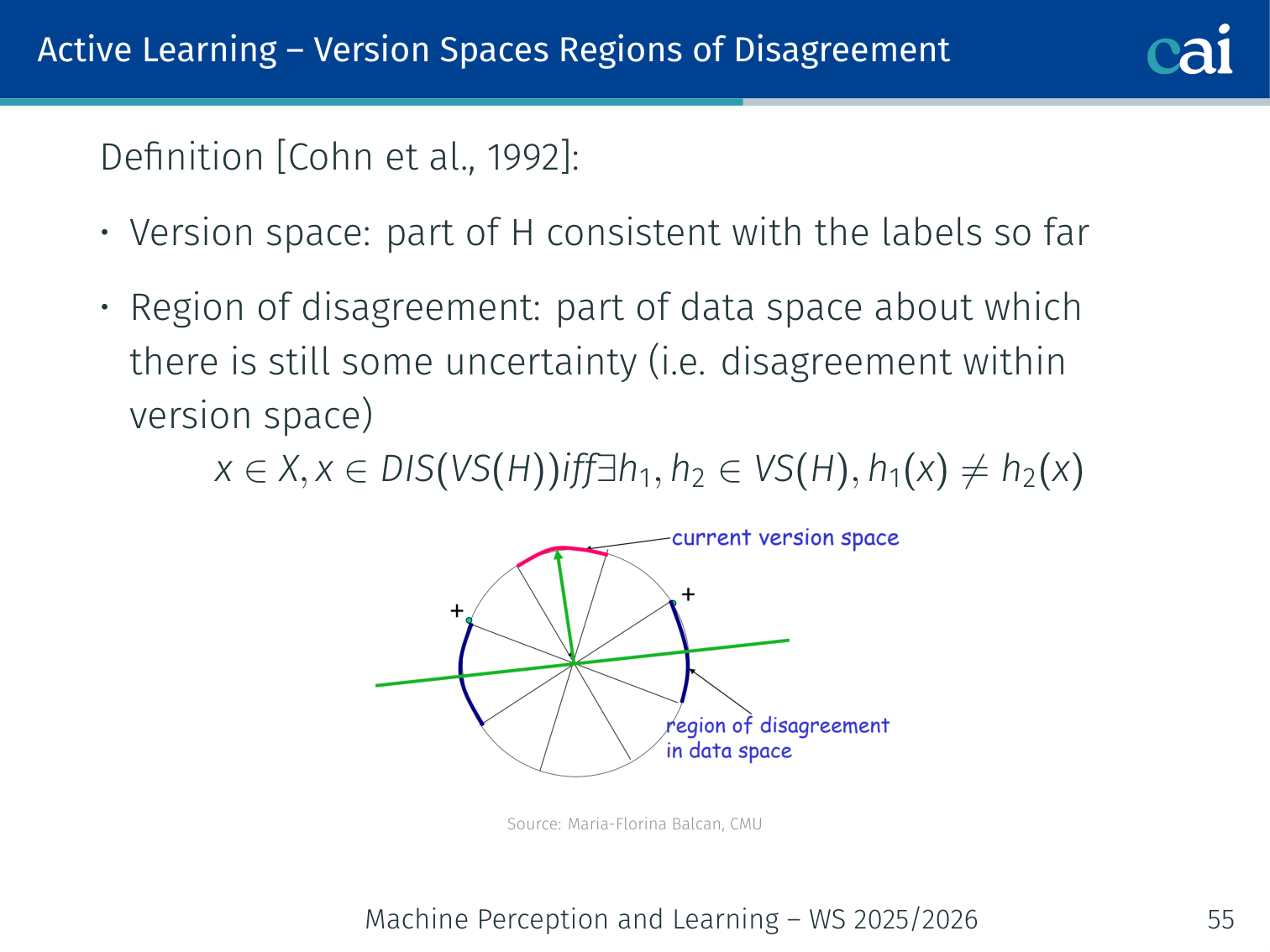
The region of disagreement where our hypotheses just can't agree on a label.

Definition (Cohn et al., 1992):

A point $x\in X$ is in the region of disagreement $DIS(VS(H))$ iff there exist $h_1,h_2\in VS(H)$ such that $h_1(x)\ne h_2(x)$:

$x\in DIS(VS(H))⟺\exists h_1,h_2\in VS(H),h_1(x)\ne h_2(x)$

Outside the region of disagreement, all hypotheses agree — labeling such a point wastes the oracle’s time.

---

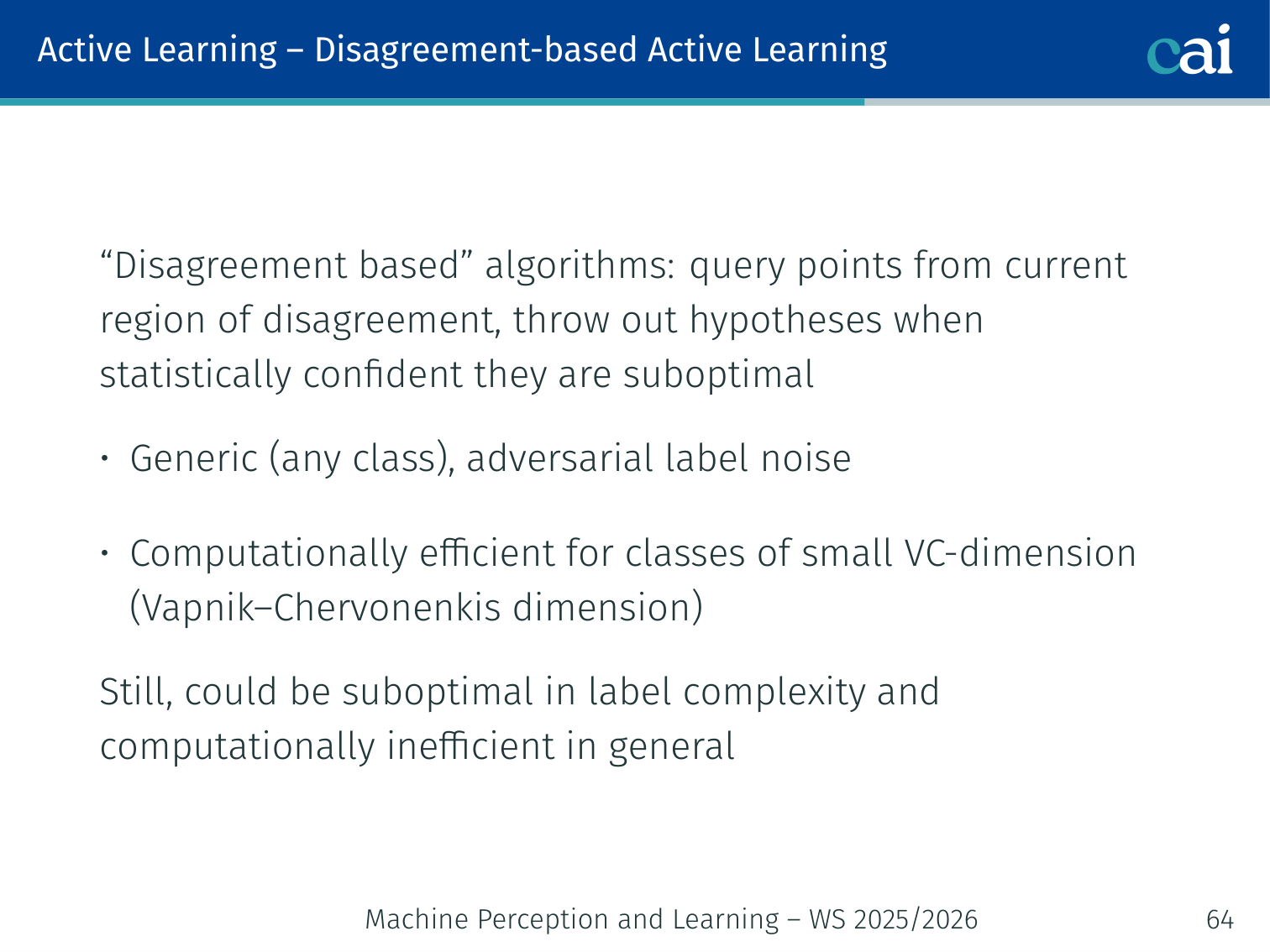
Disagreement-Based Active Learning

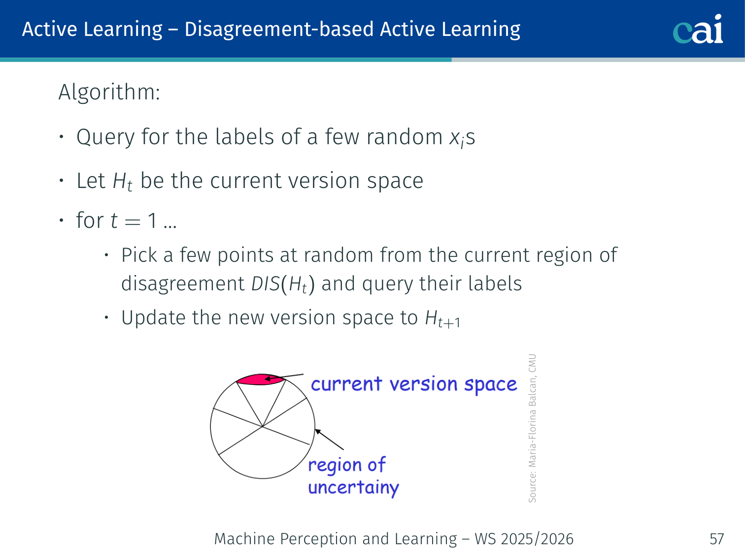
The CAL algorithm: focusing our queries on that region of disagreement.

Algorithm (CAL — Cohn et al., 1992):

1. Query labels for a few random $x_i$; initialize version space $H_1=H$
2. For $t=1,2,\dots$:
   • Pick points at random from the current region of disagreement $DIS(H_t)$
   • Query their labels
   • Update version space: $H_{t+1}\leftarrow$ hypotheses in $H_t$ still consistent with new labels
3. Stop when the region of disagreement is small

Why active? We never waste labels querying outside $DIS(H_t)$ — only queries inside can update the version space.

Example: Spam classifier with a linear decision boundary.

• After 10 labels, the version space = all lines dividing those 10 emails correctly.
• Region of disagreement = the “strip” of emails near the boundary where different consistent classifiers disagree.
• We only query emails inside that strip, not emails far away that every consistent classifier already agrees on.

---

Agnostic Active Learner — A² Algorithm

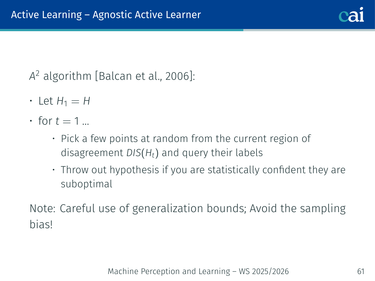
The A² Agnostic Active Learner, designed for when things get noisy or mismatched.

What if $c^{\ast }\notin H$? (The realistic case — noise, model mismatch.)

A² algorithm (Balcan, Beygelzimer, Langford, 2006):

1. Let $H_1=H$
2. For $t=1,2,\dots$:
   • Pick random points from $DIS(H_t)$, query their labels
   • Throw out any hypothesis you are statistically confident is suboptimal (using generalization bounds)
3. Avoids sampling bias by careful use of generalization bounds

Guarantees:

• Safe: never worse than passive learning
• Exponential improvement for threshold classifiers in low-noise settings
• For homogeneous linear separators in ${\mathbb{R}}^d$, uniform distribution, low noise: only $d^2\log (1/\epsilon )$ labels needed

Theoretical Guarantees — What to Retain

Theoretical guarantees and safety for disagreement-based active learning.

The lecture’s theory slides emphasise that disagreement-based active learning is attractive because it comes with explicit guarantees, not just heuristics:

• In favorable low-noise settings, active learning can provide exponential label savings
• A² is safe in the sense that it should not perform worse than passive learning
• Disagreement-based methods are quite generic and can be made computationally efficient for classes with small VC-dimension
• But they are not universally optimal: label complexity can still be suboptimal, and general computation can become expensive

---

Other AL Techniques in Practice

1. Uncertainty Sampling

A few ways to sample by uncertainty: least confidence, margin, and entropy.

Query the example the model is least confident about.

$x^{\ast }=\arg {\min }_x{\max }_{c}P(c\mid x)\text{(least confidence)}$

Or equivalently, maximise entropy:

$x^{\ast }=\arg {\max }_x-{\sum }_{c}P(c\mid x)\log P(c\mid x)$

Example: 3-class image classifier (cat / dog / bird).

• Image A: $P=[0.95,0.03,0.02]$ → entropy ≈ 0.24 → confident → skip
• Image B: $P=[0.35,0.34,0.31]$ → entropy ≈ 1.58 → very uncertain → query

2. Maximal Diversity Sampling

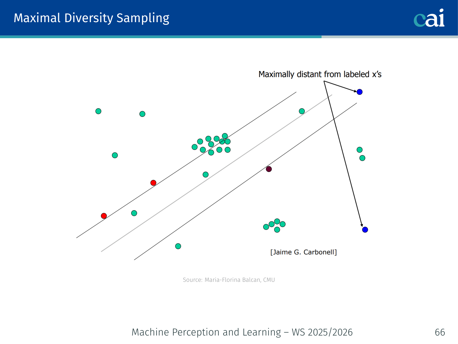
Using maximal diversity sampling to make sure we cover the whole feature space.

Select a batch of points that maximally covers the feature space, so no two queries are near-duplicates. Useful when you must query a whole batch at once.

$\text{select }B\text{ points s.t. every unlabeled point is close to at least one selected point}$

3. Ensemble-Based Possibilities (Query by Committee)

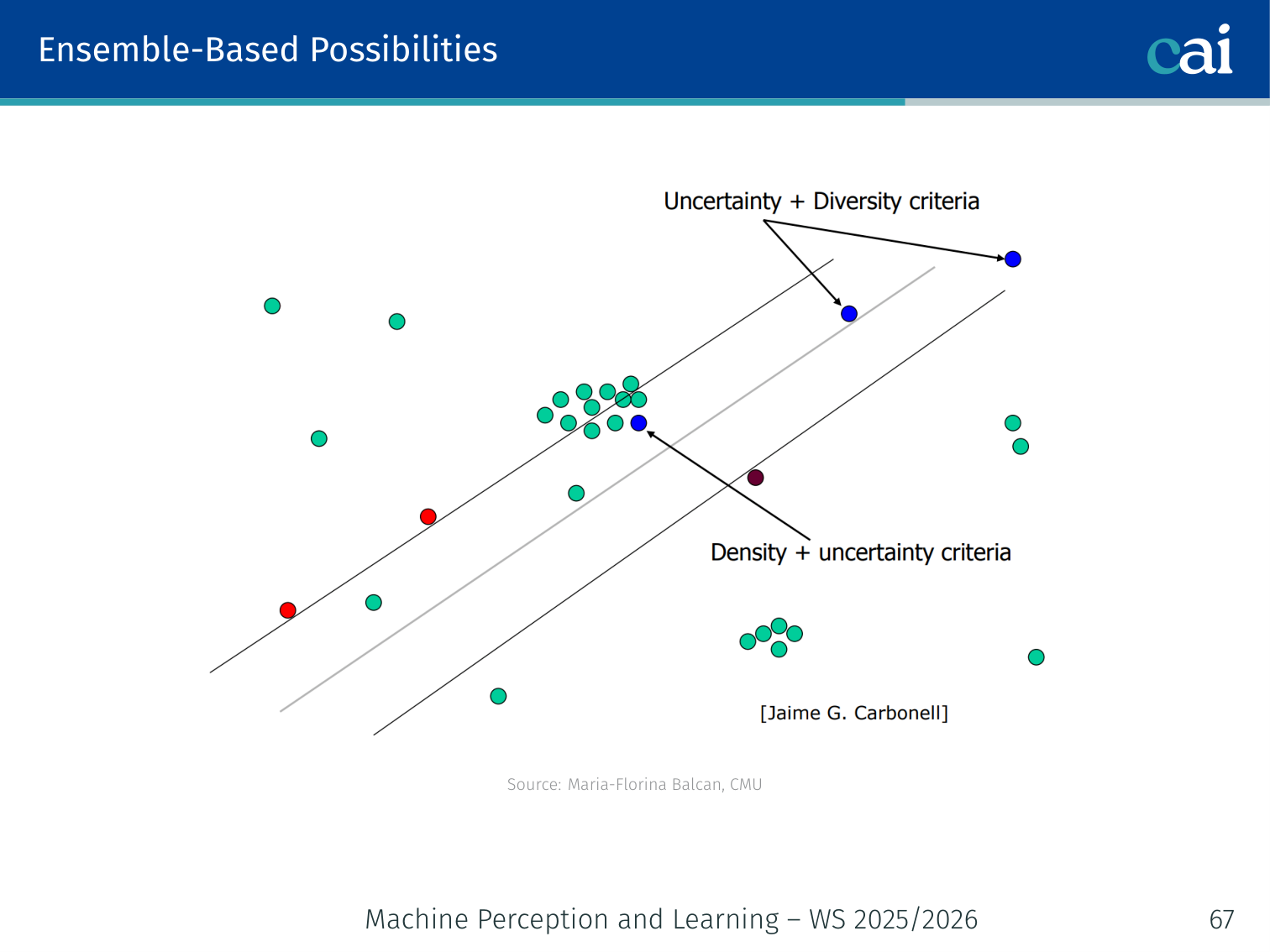
Query by Committee: letting an ensemble pick where the disagreement is highest.

Train multiple diverse models (a “committee”). Query the example where they disagree most.

The committee can be created through different initialisations, bootstrap resampling, different architectures, or approximate Bayesian samples. The key idea is always the same: if several plausible models disagree, the example is informative.

# 3-model committee
predictions = [model.predict(X_unlabeled) for model in committee]
votes = np.stack(predictions, axis=1)  # (N, C)
# Disagreement = 1 - (max vote count / num committee members)
disagreement = np.apply_along_axis(
    lambda v: 1 - np.max(np.bincount(v)) / len(v),
    axis=1, arr=votes
)
query_idx = np.argmax(disagreement)

4. Density-Based Sampling

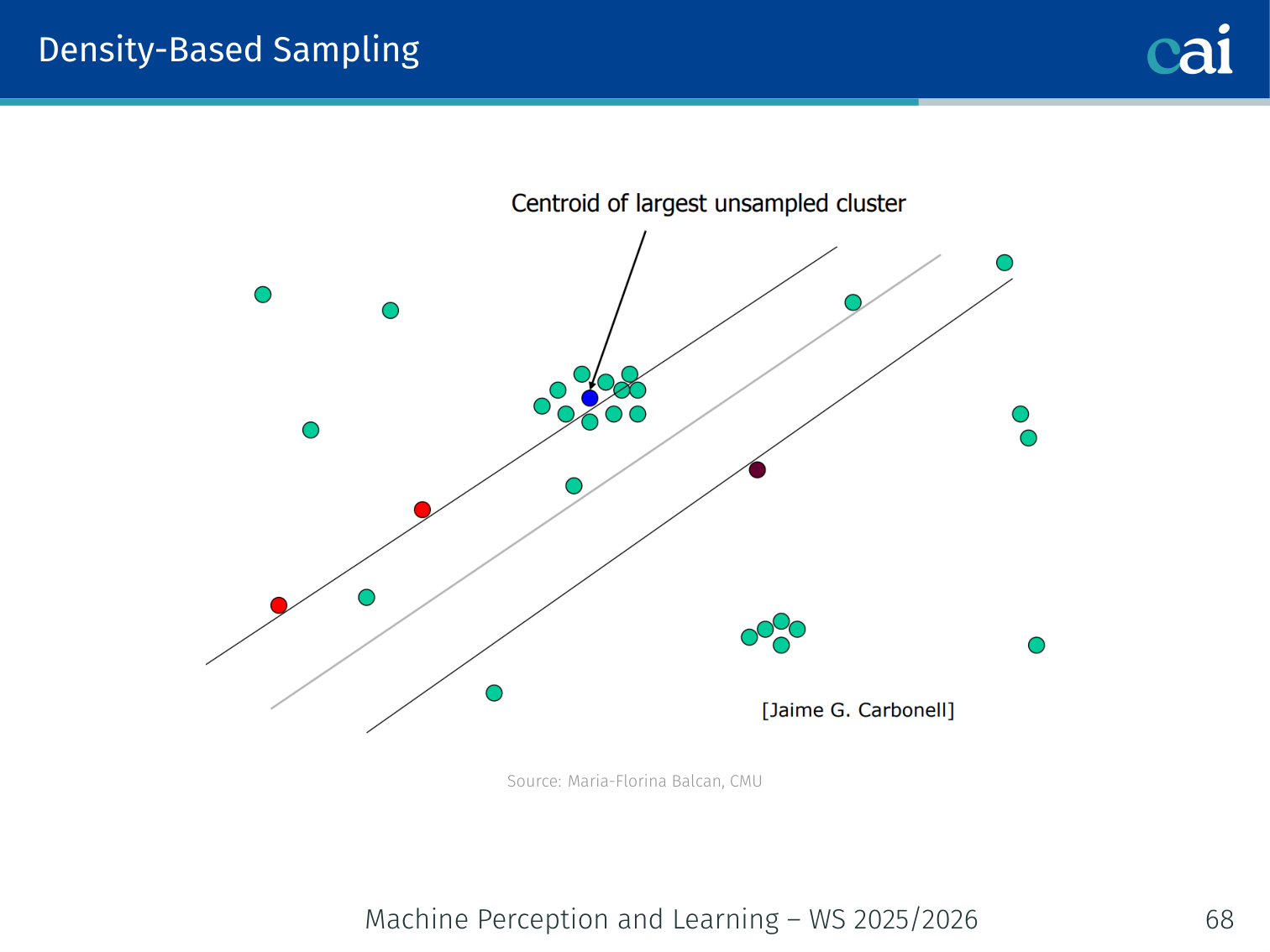
Density-based sampling: balancing uncertainty with how representative the data is.

Don’t just query uncertain points — query uncertain points that are also representative of the distribution. An uncertain but isolated point is not worth querying.

$x^{\ast }=\arg {\max }_x\text{uncertainty}(x)\times {\left(\frac{1}{U}{\sum }_u\text{sim}(x,x_u)\right)}^{\beta }$

The second term is the average similarity to all unlabeled points — a proxy for density.

---

Graph-Based Active and Semi-supervised Methods

Core Idea

Assume a pairwise similarity function exists and that very similar examples probably share the same label.

• Many labeled points → Nearest-Neighbour classifier
• Many unlabeled points → use them as “stepping stones” via label propagation

Unlabeled data can help “glue” objects of the same class together even when there is no direct edge between labeled points of the same class.

This graph view is particularly useful when the geometry of the unlabeled data is more informative than individual feature vectors: once the graph captures the manifold or cluster structure, labels can propagate through the unlabeled region instead of relying only on isolated supervised points.

Building the Graph

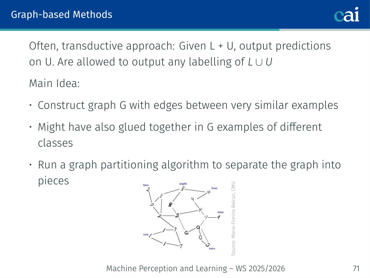
Building a similarity graph to propagate labels between nodes.

• Nodes: all examples (labeled + unlabeled)
• Edges: between very similar examples ($k$-NN or $\epsilon$-ball with Gaussian similarity weights)
• Labeled nodes have fixed labels; unlabeled nodes get soft labels via propagation

Often used in a transductive setting: given $L\cup U$, output predictions on $U$ (not required to generalize to brand-new test points).

Graph Partitioning Algorithms

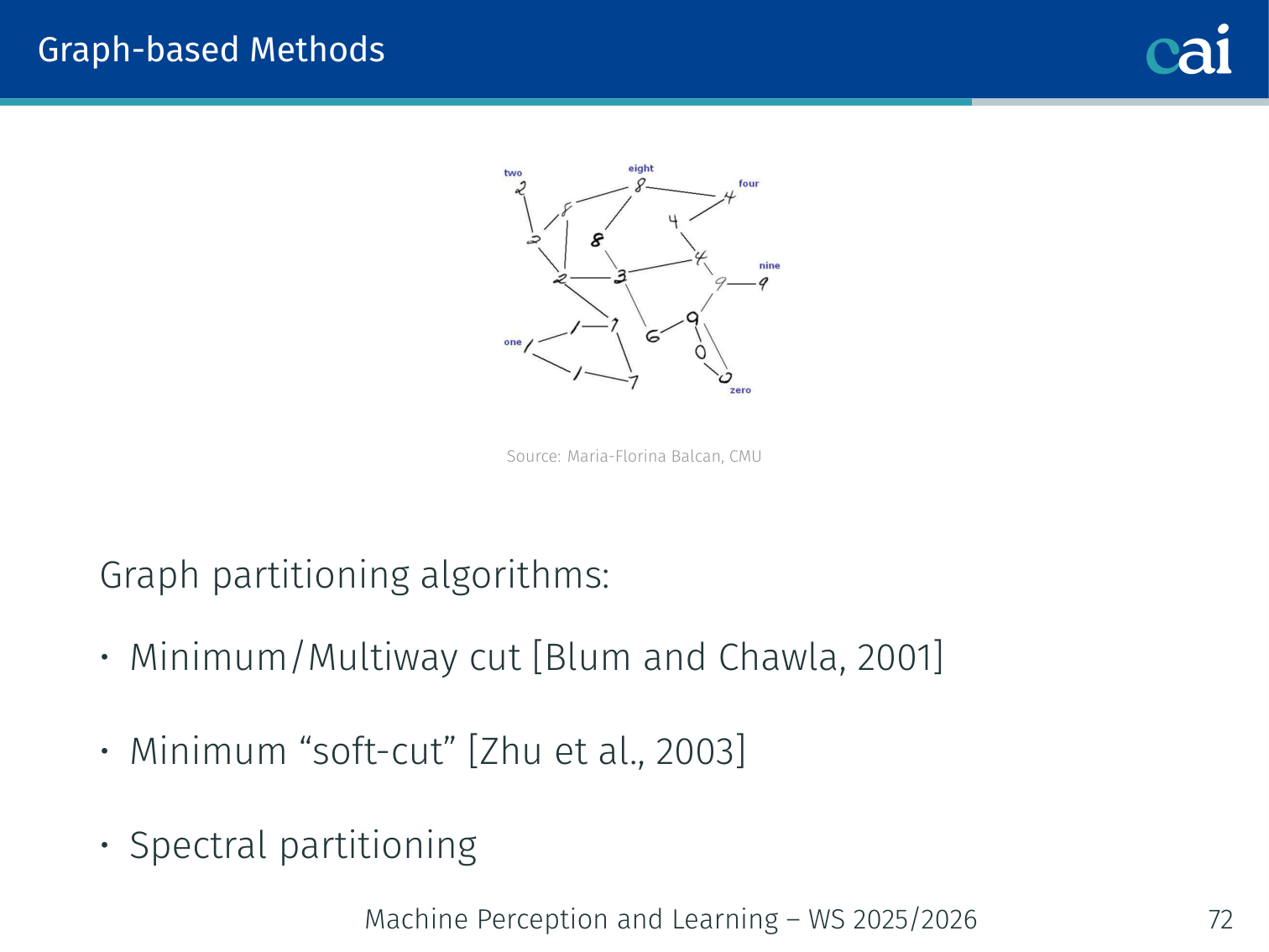
Comparing graph partitioning: min-cut, soft-cut, and spectral methods.

Method	Description
Minimum cut (Blum & Chawla, 2001)	Hard partition: minimize total weight of cut edges
Soft cut / Label propagation (Zhu et al., 2003)	Smooth label function minimizing ${\sum }_{ij}{w}_{ij}(f(x_i)-f(x_j){)}^2$
Spectral partitioning	Eigenvectors of the graph Laplacian

Semi-supervised Learning with Soft Cuts (Zhu et al., 2003)

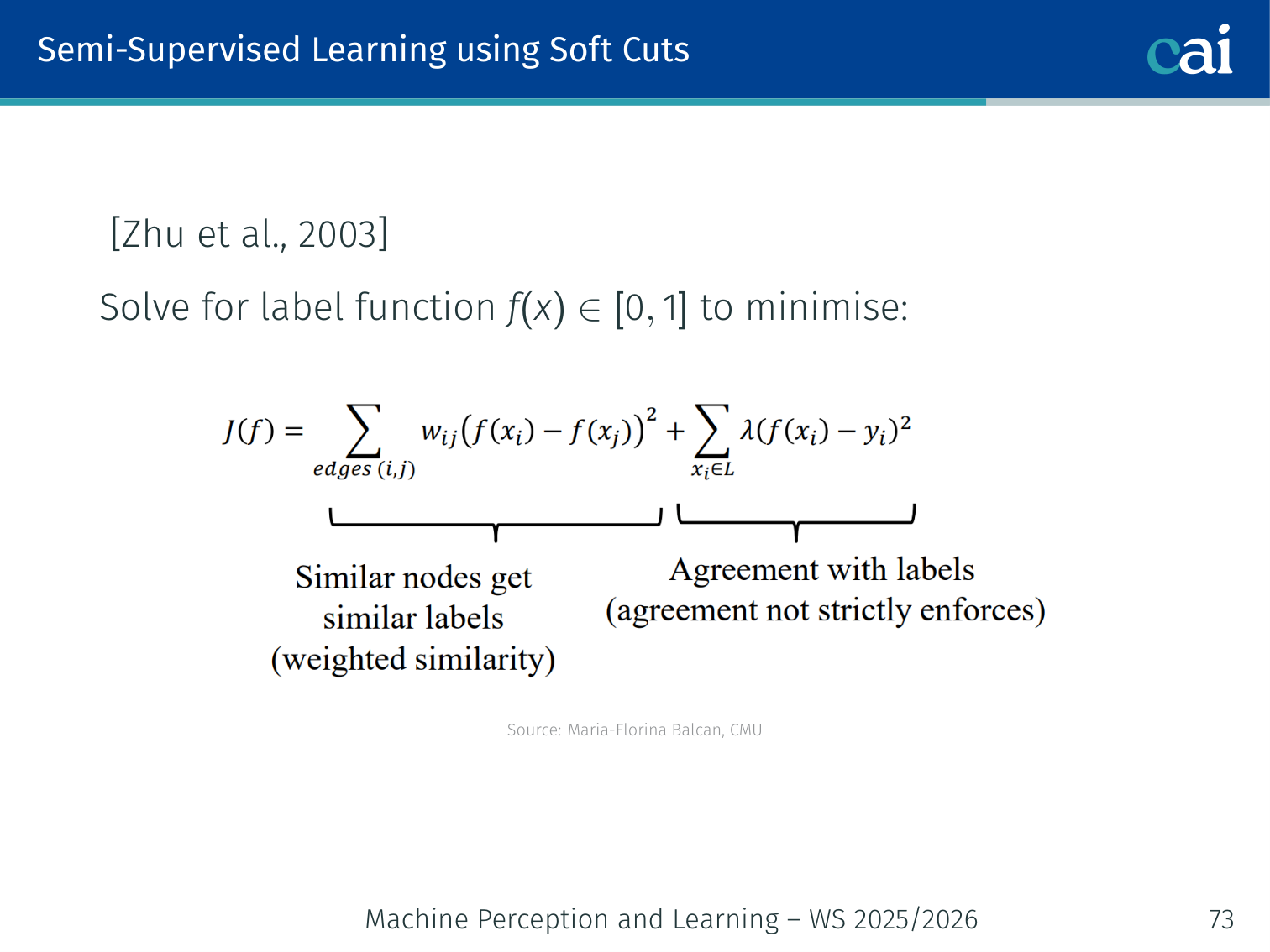
Label propagation works like a harmonic function spreading through the graph.

Solve for a label function $f(x)\in [0,1]$ that minimises:

${\min }_f{\sum }_{i,j}{w}_{ij}(f(x_i)-f(x_j){)}^2\text{subject to }f(x_i)=y_i\text{ for labeled nodes}$

This is a harmonic equation: labels spread outward from labeled nodes, weighted by edge similarity. The solution can be found by solving a sparse linear system.

Example: A document graph where edges connect articles sharing many keywords. Label 3 articles in a “sports” cluster as positive and 2 articles in a “finance” cluster as negative. Label propagation will assign positive labels to all sports articles and negative to all finance articles, flowing through the keyword-similarity edges.

Active Learning with Label Propagation

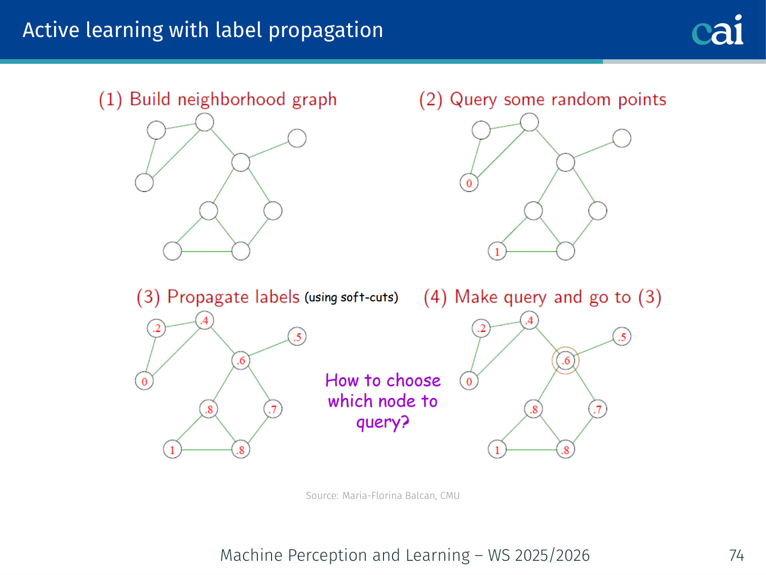
An active learning strategy for graphs: query nodes that spread the most info.

The 1-step lookahead heuristic for picking the best nodes to label.

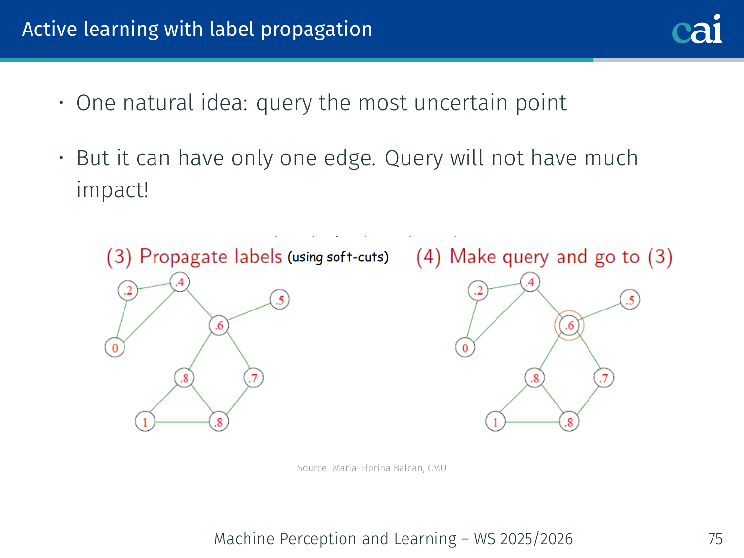
Naïve approach: query the node with $f(x)\approx 0.5$ (most uncertain).

Problem: The uncertain node might be nearly isolated (just one edge) — labeling it won’t propagate much information.

Better — 1-step lookahead heuristic (Fathi et al., 2011):

For each candidate node $s$ with current soft label $p$:

1. Assume the oracle answers $1$ with probability $p$, answers $0$ with probability $1-p$
2. Run label propagation for each outcome, compute average confidence across all nodes
3. Query the node that maximises expected confidence:

$\text{score}(s)=p\cdot \frac{1}{n}{\sum }_i\max (f_1(x_i),1-f_1(x_i))+(1-p)\cdot \frac{1}{n}{\sum }_i\max (f_0(x_i),1-f_0(x_i))$

This approach performs well for video segmentation (Fathi et al., 2011) where frames are nodes and edge weights come from visual similarity.

---

Deep Active Learning

Deep Active Learning: it's tricky with softmax confidence and batching.

Deep active learning is best viewed as a continuation of the classical ideas, not a separate topic. The same goals remain:

• estimate uncertainty
• capture disagreement
• avoid redundant batch queries
• prefer points that influence the rest of the pool

What changes is that deep networks do not expose these quantities cleanly, so we need approximations such as MC Dropout, BALD, and batch-aware acquisition objectives.

Challenges

Classical active learning theory assumes a fixed, well-understood hypothesis class. DNNs break this:

1. Overconfident softmax: the softmax output of DNNs is typically overconfident — high probability outputs even on misclassified examples
2. Batch selection: large-scale training requires selecting a batch of images at once, not one at a time
3. Mode collapse: uncertainty heuristics may repeatedly select examples from the same class, severely imbalancing the training set

---

MC Dropout — Bayesian Approximation

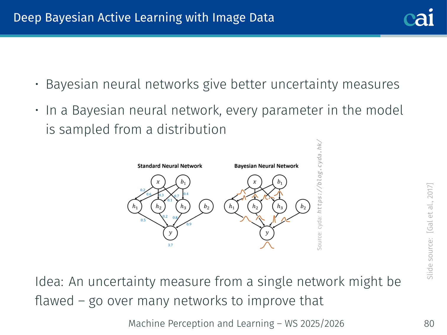
Approximating Bayesian uncertainty using MC Dropout at test time.

(Gal et al., 2017) In a Bayesian neural network, every weight is a distribution. Integrating over all parameters is intractable:

$p(y=c\mid x)=\int p(y=c\mid x,\omega )p(\omega )d\omega$

Approximation via MC Dropout:

• Apply dropout at test time (not just during training)
• Run $T$ forward passes with different dropout masks — each pass samples a “thinned” network
• Average predictions:

$p(y\mid x)\approx \frac{1}{T}{\sum }_t{p}_c^t$

The variance across runs captures uncertainty.

model.train()  # keep dropout active at test time
T = 50
 
preds = np.stack([
    model(x).softmax(-1).detach().cpu().numpy()
    for _ in range(T)
])  # shape: (T, N, C)
 
mean_pred = preds.mean(axis=0)  # (N, C)
entropy = -(mean_pred * np.log(mean_pred + 1e-8)).sum(axis=1)  # (N,)
query_indices = entropy.argsort()[-batch_size:]

High entropy → every dropout run is confident about a different class → very uncertain → good to query.

---

BALD — Bayesian Active Learning by Disagreement

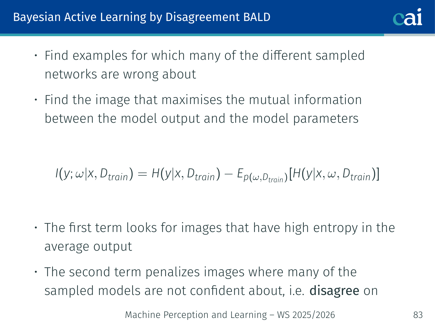
The BALD strategy: find where models are confident but totally disagree.

(Gal et al., 2017) — more principled than pure entropy:

$I(y;\omega \mid x,\mathcal{D})=\underset{\text{entropy of mean}}{\underbrace{H(y\mid x,\mathcal{D})}}-\underset{\text{mean entropy of individual models}}{\underbrace{{\mathbb{E}}_{p(\omega \mid \mathcal{D})}[H(y\mid x,\omega ,\mathcal{D})]}}$

• First term: high if the average model output is uncertain
• Second term: penalises cases where individual models are also uncertain — we want models that are individually confident but disagree with each other

$x^{\ast }=\arg {\max }_{x}I(y;\omega \mid x,\mathcal{D}$

In practice with MC Dropout:

$I\approx -{\sum }_c\left(\frac{1}{T}{\sum }_t{p}_c^t\right)\log \left(\frac{1}{T}{\sum }_t{p}_c^t\right)+\frac{1}{T}{\sum }_t{\sum }_c{p}_c^t\log p_c^t$

Example: Blurry image of a handwritten digit — looks like either 4 or 9.

• Entropy: average of 50 dropout runs gives $[0.5,0.5]$ (4 vs 9) → high uncertainty ✓
• Expected entropy: each individual run says “definitely 4” or “definitely 9” → low — models are confident individually but disagree → high BALD score → query this image

---

Learning Loss for Active Learning

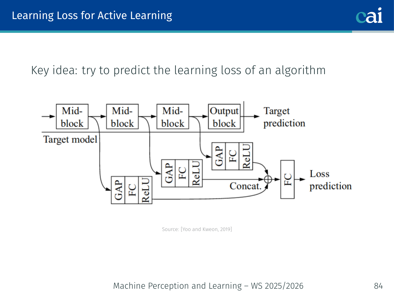
Learning to predict loss with an extra module to help pick samples.

Using pairwise ranking to keep the loss prediction module training stable.

(Yoo & Kweon, 2019) — predict which examples the model will get wrong.

Architecture:

• Extract intermediate features from multiple layers of the main network
• A small auxiliary loss prediction module combines them and outputs a predicted loss for each unlabeled example
• Query examples with the highest predicted loss

Challenge: loss values change as the model trains. Instead of regressing the raw loss value, compare pairs:

• Split each batch of size $B$ into $B/2$ pairs
• For each pair, predict which image has the higher loss
• Train with a pairwise ranking loss (more stable)

---

Mode Collapse in Active Learning

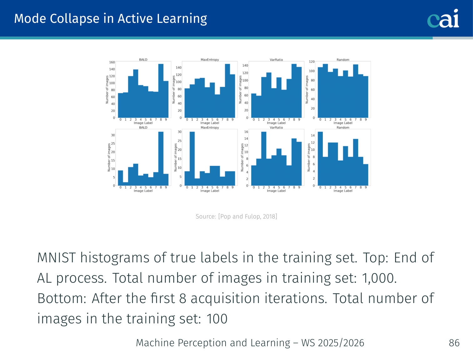
Mode collapse in action: over-sampling those tricky classes like 4 vs 9.

A critical failure mode: the uncertainty-based strategy keeps selecting the same hard class, resulting in a severely imbalanced training set.

Observed on MNIST (Pop & Fulop, 2018): After active learning with 1,000 queried images, the set contains many “hard” digits (4 vs 9 are easily confused) and very few “easy” digits (1, 0). The model then performs poorly on the easy digits.

---

Batch-Aware Methods — Uncertainty vs. Diversity (BatchBALD)

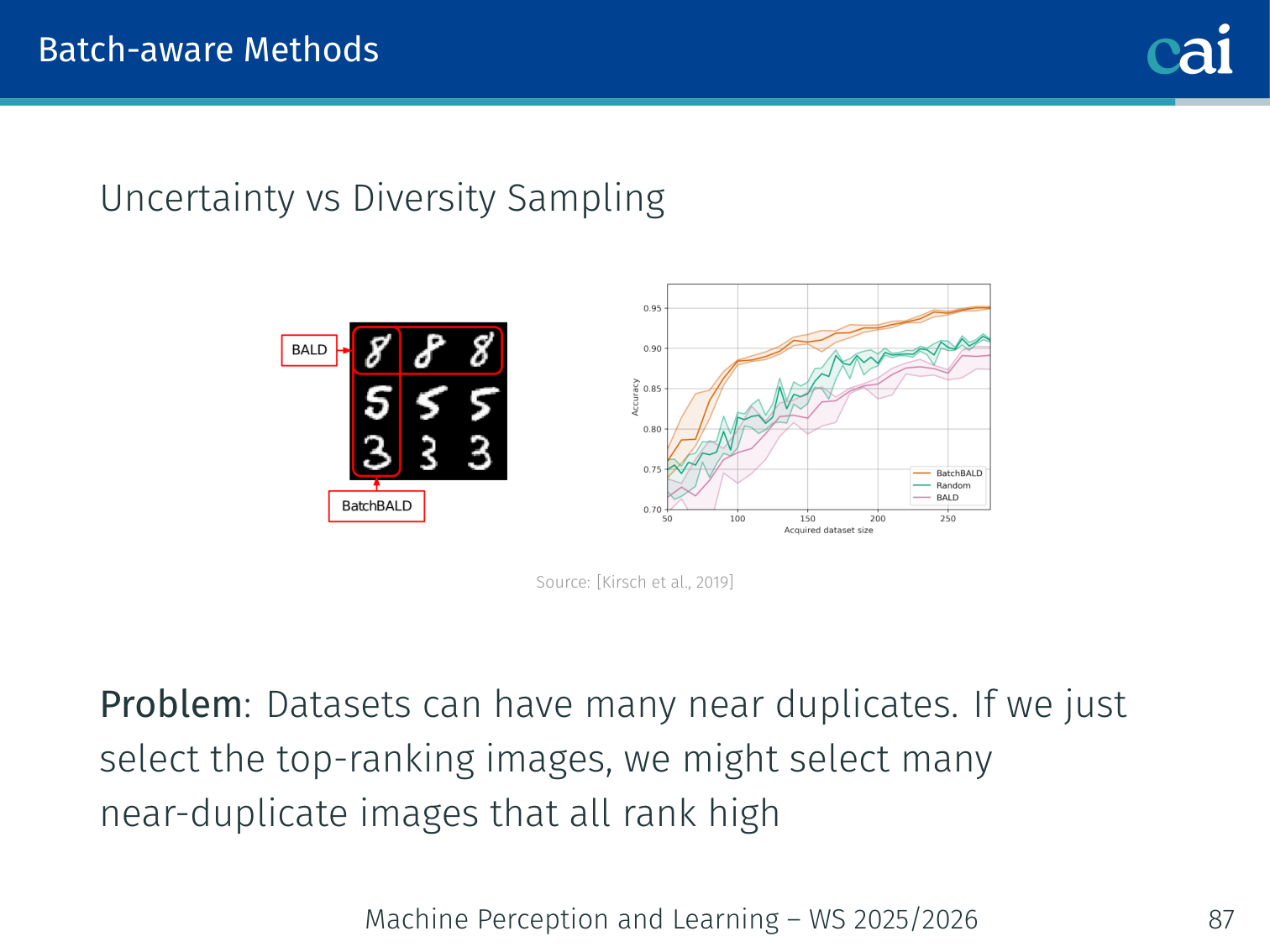
Comparing strategies for batch acquisition: uncertainty, diversity, and BatchBALD.

(Kirsch, van Amersfoort, Gal — NeurIPS 2019)

Problem: Ranking all unlabeled examples by uncertainty and picking the top-$B$ grabs many near-duplicate images. Real datasets have many images that are visually almost identical — wasting the labeling budget.

Solution: Maximise the joint mutual information of the entire queried batch with the model parameters — this naturally penalises redundancy:

$x_1^{\ast },\dots ,x_B^{\ast }=\arg \max I(y_1,\dots ,y_B;\omega \mid x_1,\dots ,x_B,\mathcal{D})$

Uncertainty alone grabs near-duplicates; diversity alone ignores which regions are actually uncertain. BatchBALD balances both.

---

Summary

Short Summary

A quick wrap-up of iML techniques and what makes them tick.

• Active learning can deliver exponential improvements in label complexity, both in theory and practice
• Common heuristics (uncertainty sampling, active SVM) work but beware of sampling bias
• Disagreement-based safe schemes (A²) provide noise-robust guarantees
• Graph methods leverage data manifold structure for label propagation
• Deep active learning reuses the same principles with approximate Bayesian uncertainty and batch-aware objectives

Techniques at a Glance

Technique	Core Idea	Key Risk
Uncertainty sampling	Query least-confident examples	Sampling bias
Disagreement-based (A²)	Query within version space’s region of disagreement	Computationally expensive in general
Maximal diversity / Core-Set	Batch covering feature space	Ignores uncertainty
Query by committee	Query where committee disagrees most	Needs diverse committee
Density-based	Weight uncertainty by representativeness	Density estimation cost
Graph label propagation	Labels flow through similarity graph	Needs good similarity metric
MC Dropout / BALD	Bayesian uncertainty via multiple forward passes	$T$ forward passes per query round
Learning Loss	Predict which examples have high loss	Auxiliary module complexity
BatchBALD	Joint MI maximisation for batch acquisition	Computationally intensive
Semi-supervised (soft cuts)	Harmonic label propagation on unlabeled data	Requires compatible distribution assumption

PyTorch Implementation: Graph Neural Network (Sudoku Solver)

While standard MLPs and CNNs struggle with the long-range constraints of Sudoku, Graph Neural Networks (GNNs) solve the puzzle by treating cells as nodes and the rules of the game (rows, columns, boxes) as explicit edges.

See the full project: (y-) Case Study: Sudoku GNN.

Mental Model: Iterative Reasoning via Message Passing

• Think of each cell in a Sudoku board as a reasoning agent.
• At each timestep, every agent looks at its neighbors (cells in the same row, column, or 3x3 box) and asks: “What numbers are you already sure about?”
• The agent updates its own internal “belief” based on these messages.
• After $T$ iterations, this local communication propagates information across the entire board, allowing the network to “solve” the global puzzle.

💡 Intuition: Why GNNs beat CNNs at Sudoku

• A CNN is limited by its receptive field; it can only “see” a small 3x3 or 5x5 area at a time. To see a whole 9x9 board, you need many layers.
• A GNN with explicit edges for rows and columns has a receptive field of 1 for all constraints. A cell is directly connected to every other cell that restricts its value. This “shortcut” for relational reasoning makes the learning problem significantly easier.

import torch
import torch.nn as nn
 
class GNN(nn.Module):
    def __init__(self, n_iters=7, n_node_features=10):
        super().__init__()
        self.n_iters = n_iters # Number of message-passing "reasoning" steps
 
        # 1. Message network: learns how nodes should talk to each other
        self.msg_net = nn.Sequential(
            nn.Linear(2 * n_node_features, 64),
            nn.ReLU(),
            nn.Linear(64, 11) # Outputs a 'message' vector
        )
 
        # 2. State update network: uses messages to update node belief
        # GRUCell maintains a "memory" of the node state across iterations
        self.gru = nn.GRUCell(9 + 11, n_node_features) # Input = (digit_ID + message)
 
        # 3. Output head: maps final node state to 9 digit probabilities
        self.fc_out = nn.Linear(n_node_features, 9)
 
    def forward(self, node_inputs, src_ids, dst_ids):
        """
        Args:
            node_inputs: Initial clues for each Sudoku cell (n_nodes, 9)
            src_ids, dst_ids: Indices defining row/col/box constraints
        """
        n_nodes = node_inputs.size(0)
        node_states = torch.zeros(n_nodes, 10)
 
        for _ in range(self.n_iters):
            # STEP 1: Message Passing (Gather neighbor states)
            msg_in = torch.cat([node_states[src_ids], node_states[dst_ids]], 1)
            messages = self.msg_net(msg_in)
 
            # STEP 2: Aggregation (Sum incoming messages)
            agg_msg = torch.zeros(n_nodes, 11)
            agg_msg.index_add_(0, dst_ids, messages)
 
            # STEP 3: State Update (Update belief using GRU)
            node_states = self.gru(torch.cat([node_inputs, agg_msg], 1), node_states)
 
        return self.fc_out(node_states)

Key GNN Concepts:

• Local to Global: Information from the other side of the board propagates via multiple steps.
• Permutation Invariance: The index_add_ (sum) operation ensures result consistency regardless of neighbor order.
• Relational Reasoning: The model learns the rules of Sudoku encoded in the graph structure.

Applied Exam Focus

• Uncertainty Sampling: In Active Learning, query points where the model is least confident (e.g., Highest Entropy or Smallest Margin between top two classes).
• Label Propagation: Uses a Similarity Graph to spread labels from a few points to many. It assumes that points close on the graph manifold share the same label.
• GNN Iterations: Each message-passing step increases the receptive field by one hop. To capture a whole Sudoku board, you need at least $T=9$ iterations.

---

Previous: L07 — Multimodal | Back to MPL Index | Next: (y-09) VAE | (y) Return to Notes | (y) Return to Home