L09 — Generative AI & Variational Autoencoders (VAE)

Previous: L08 — IML | Back to MPL Index | Next: (y-10) GANs

Slide credits: O. Hilliges @ ETHZ · Paul Liang & Louis-Philippe Morency @ CMU

---

Mental Model First

• A VAE is a probabilistic autoencoder: it wants to reconstruct data while also shaping the latent space so we can sample from it.
• Plain autoencoders compress well, but their latent spaces are usually messy and unreliable for generation.
• The KL term is what turns a useful compression model into a generative model with a smoother, more navigable latent space.
• If one question guides this lecture, let it be: how can we force a latent representation to be both informative for reconstruction and structured enough for sampling?

Introduction

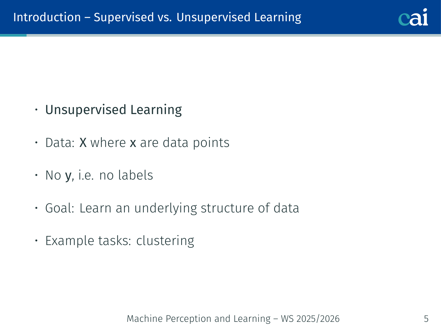
Supervised vs. Unsupervised Learning

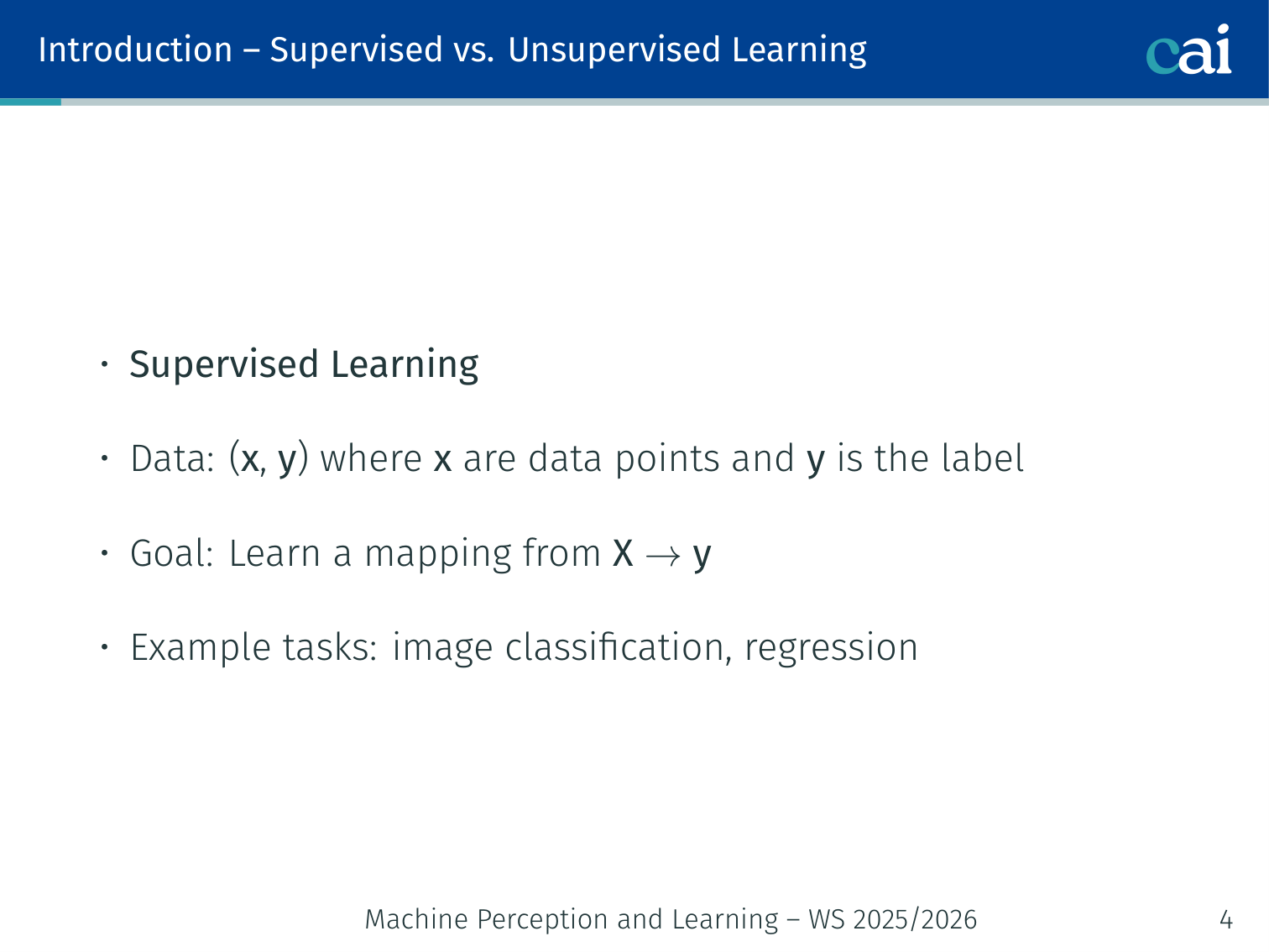
Supervised vs. unsupervised: the difference between having labels and going it alone.

A quick look at the goals for supervised and unsupervised learning.

	Supervised	Unsupervised
Data	$(x,y)$ — labelled pairs	$x$ — no labels
Goal	Learn mapping $X\to y$	Learn underlying structure of data
Examples	Image classification, regression	Clustering, generation

Generative Modelling

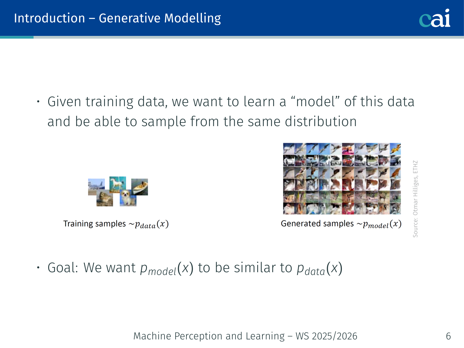
Generative modeling in a nutshell: learning to sample from our data distribution p(x).

Given training data, we want to learn a model of the data and be able to sample from the same distribution.

$p_{\text{model}}(x)\approx p_{\text{data}}(x)$

What we want to do with $p_{\text{model}}(x)$:

• Evaluate $p_{\text{model}}(x)$ — realistic data should score high, fake data should score low
• Sample new $x\sim p_{\text{model}}(x)$ — e.g. generate realistic images

We may also want conditional generation $p(x|c)$, where $c$ is a category (e.g. “generate a face”), or even $p(x_2|x_1,c)$ for style transfer (change style $c$ applied to image $x_1$).

Latent Variable Models

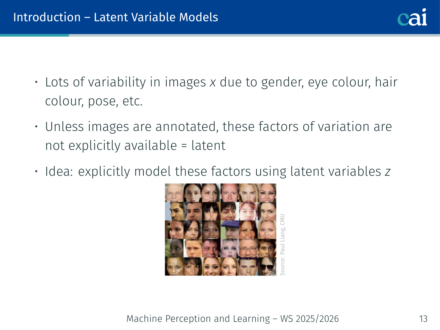
Modeling those hidden factors of variation using latent variables.

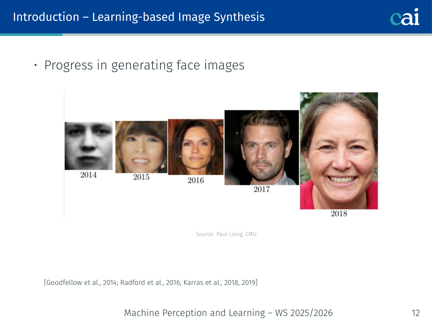
Images have huge variability: gender, eye colour, hair colour, pose, lighting, etc. Unless annotated, these factors of variation are not explicitly available — they are latent.

Idea: explicitly model these factors with latent variables $z$.

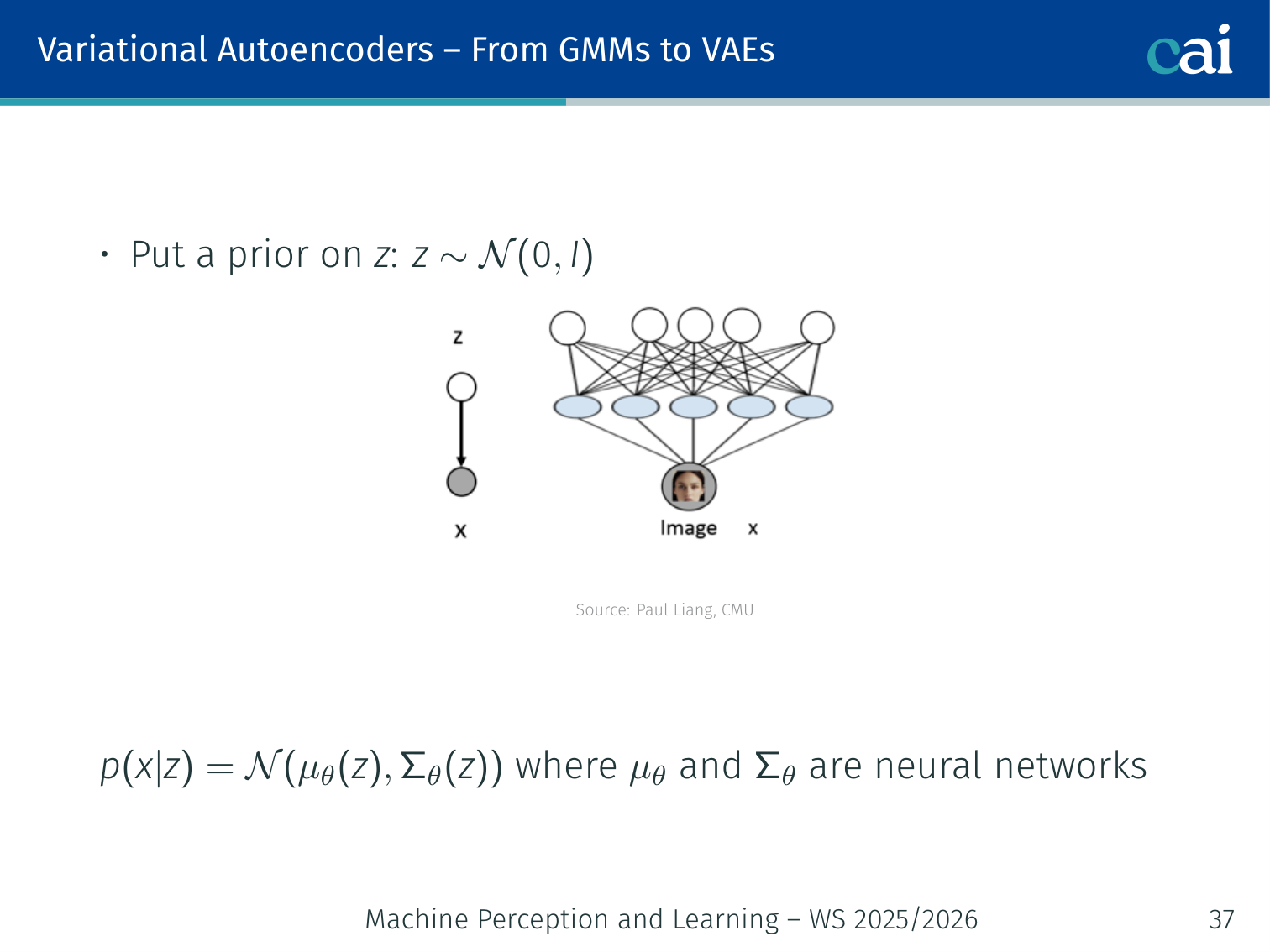
• Put a prior on $z$: $z\sim \mathcal{N}(0,I)$
• Model the data with: $p(x|z)=\mathcal{N}({\mu }_{\theta }(z),{\Sigma }_{\theta }(z))$ where ${\mu }_{\theta }$ and ${\Sigma }_{\theta }$ are neural networks
• After training, $z$ should correspond to meaningful factors — hair colour, pose, etc.
• Given a new image $x$, extract features via $p(z|x)$ — useful for clustering and representation learning

Example: two images of the same person smiling will map to nearby $z$ vectors; an image of a different person with the same pose will share some $z$ dimensions but differ in others.

Maximum Likelihood Estimation (MLE)

MLE: the foundational goal for pretty much all deep learning models.

Likelihood as a function of model parameters:

$L(\theta )={\prod }_{i}p(x_i|\theta )⟹\log L(\theta )={\sum }_i\log p(x_i|\theta )$

MLE is the backbone of supervised deep learning — cross-entropy and least-squares are both MLE estimators. Generative models extend this to the unsupervised setting.

Taxonomy of Generative Models

How we group generative models: explicit density vs. implicit ones.

Generative Models
├── Explicit Density (define p(x) explicitly)
│   ├── Tractable density
│   │   ├── Auto-regressive  (PixelCNN, WaveNet)
│   │   └── Flow models      (RealNVP, Glow)
│   └── Approximate density
│       ├── VAE              (variational inference)
│       └── Diffusion models (DDPM, DDIM)
└── Implicit / Likelihood-free
    └── GANs (generator + discriminator)

Explicit models define $p(x)$ and evaluate likelihoods → MLE training. Implicit / likelihood-free models (GANs) are highly expressive but the density function is not defined or is intractable — basis for adversarial training. [Goodfellow et al., 2014; Radford et al., 2016; Karras et al., 2018, 2019]

---

Mixture of Gaussians (MoG)

A Mixture of Gaussians: a simple example of a latent variable model.

A simple but instructive latent variable model.

$z\sim \text{Categorical}(1\dots K),p(x|z=k)=\mathcal{N}({\mu }_k,{\Sigma }_k)$

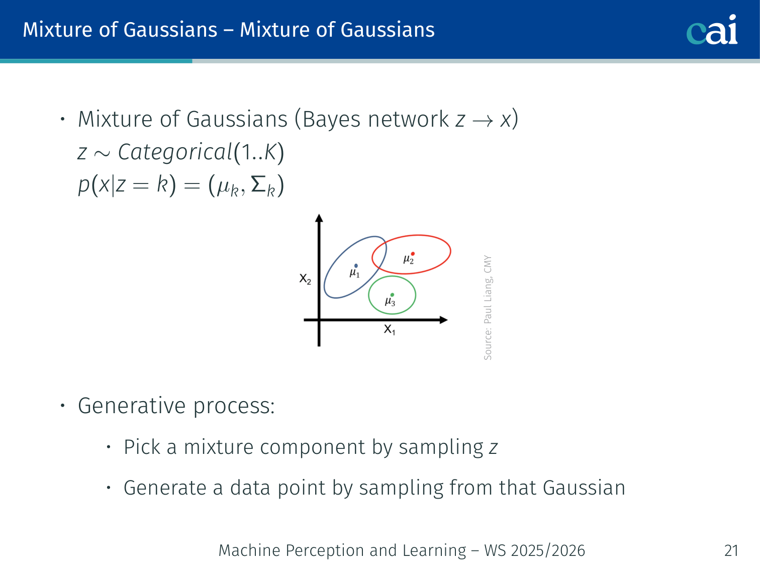
Generative process:

1. Pick a mixture component by sampling $z\sim \text{Categorical}(\pi )$
2. Sample the data point from that Gaussian: $x\sim \mathcal{N}({\mu }_z,{\Sigma }_z)$

Marginal (integrating out $z$):

$p(x)={\sum }_{z}p(x,z)={\sum }_{k=1}^{K}p(z=k)\mathcal{N}(x;{\mu }_k,{\Sigma }_k)$

Combining simple Gaussians gives a much more expressive, multi-modal density.

Example — MNIST clustering: fit a MoG with $K=10$ components to MNIST pixels. The model often discovers clusters that roughly correspond to digit identities (0–9) without ever seeing labels. You can also sample new digit images from each cluster, but the quality is low because MoG cannot learn complex pixel-level features.

Limitation: MoG cannot learn rich features of the data (it cannot compute $p(z|x)$ in a meaningful, scalable way for high-dimensional $x$ like images).

---

Autoencoders

Architecture

The standard autoencoder: an encoder, a decoder, and that latent bottleneck.

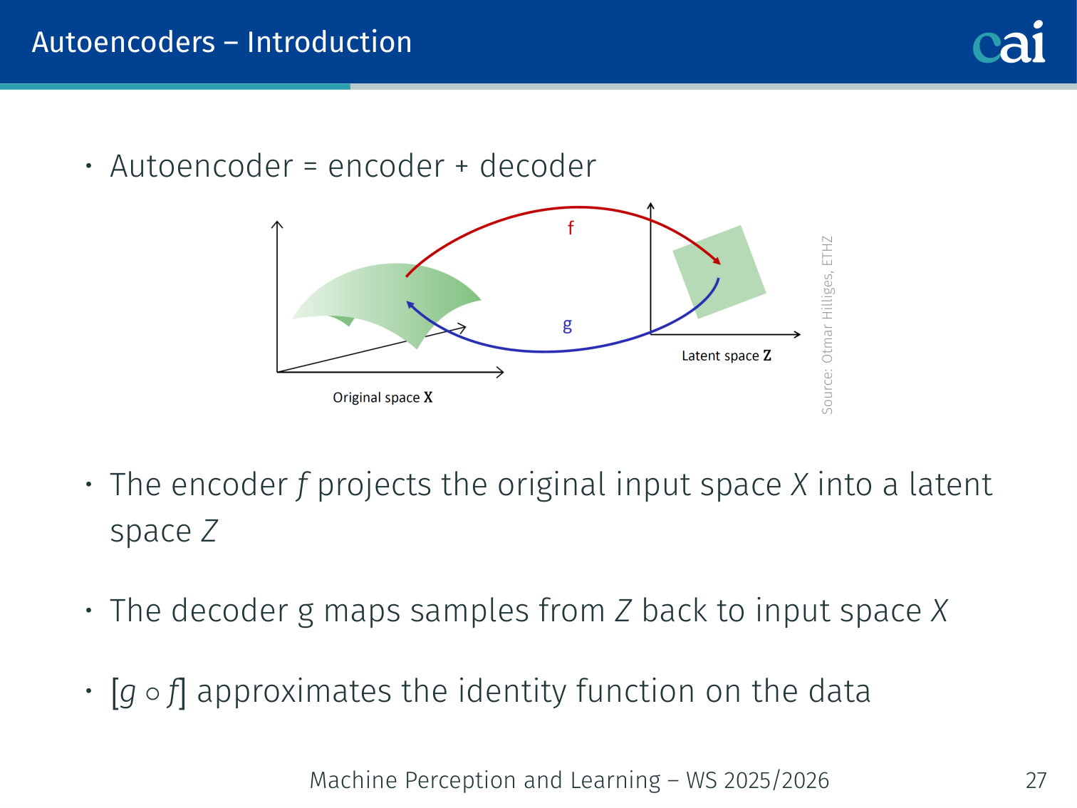
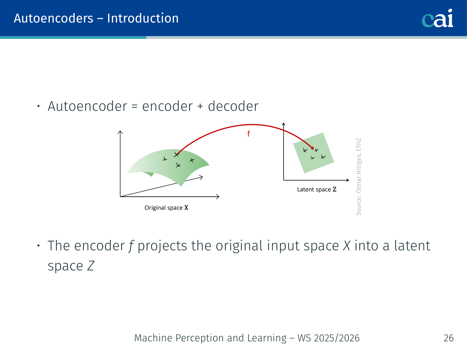
An autoencoder = encoder $f$ + decoder $g$.

x ──→ [Encoder f] ──→ z ──→ [Decoder g] ──→ x̂
       (compress)    latent    (reconstruct)

• Encoder $f$: projects input space $\mathcal{X}$ into a low-dimensional latent space $\mathcal{Z}$
• Decoder $g$: maps samples from $\mathcal{Z}$ back to $\mathcal{X}$
• Together $[g\circ f]$ approximates the identity on the data

Training objective — minimize reconstruction error:

${\hat{\theta }}_f,{\hat{\theta }}_g=\arg {\min }_{{\theta }_f,{\theta }_g}{\sum }_{n=1}^N\Vert x_n-g(f(x_n)){\Vert }^2$

Linear special case: if both $f$ and $g$ are linear, the optimal solution is PCA — the encoder learns the top-$d$ principal components.

What Autoencoders Are Good At

• Dimensionality reduction and compression
• Denoising (train on corrupted input, reconstruct clean output)
• Representation learning: use $z$ for downstream classification or clustering

Why Autoencoders Fail for Generation

After training, the latent space $\mathcal{Z}$ is irregular and discontinuous — points that decode to valid images cluster in disconnected islands. Sampling a random $z$ and decoding produces garbage.

Analogy: imagine the library stacks were randomly assigned. Opening a random drawer is unlikely to give you a coherent book.

Fitting a simple Gaussian $f(x)\sim \mathcal{N}(\hat{\mu },\hat{\sigma }I)$ over the encoded training points and sampling from it does not work either — the density model is too simple to capture the true structure.

MNIST example: plot the 2D latent codes of an autoencoder trained on MNIST. You’ll see tight clusters per digit with large empty gaps between them. A random sample from $z$-space lands in the gaps → blurry or meaningless output.

---

💡 Intuition: VAE as “Fuzzy” Compression

Think of a normal Autoencoder as a librarian who remembers the exact shelf and position for every book. If you ask for a book at a random position, they won’t know what to do.

A VAE is like a librarian who remembers the general area where each book is (e.g., “The History books are in that corner cloud”).

• When the VAE encodes an image, it doesn’t just output one point ($z$).
• It outputs a mean (the center of the cloud) and a standard deviation (the size of the cloud).
• During training, we sample a point from this cloud. This forces the model to ensure that every point in that general area decodes to something meaningful.

This “fuzziness” is what makes the latent space continuous and allows us to sample new, realistic images.

---

🧠 Deep Dive: Why the KL Divergence Penalty?

In the VAE loss, we have two parts: Reconstruction (how well it copies the input) and KL Divergence (how much the latent distribution looks like a standard Gaussian).

What happens if we remove the KL term? The model will “cheat”. It will make each cloud extremely tiny (zero variance) and move them as far apart as possible so they don’t overlap. This makes reconstruction easy, but it destroys the “fuzziness”. We end up with a normal Autoencoder where the space between clouds is empty “garbage” space.

What happens if the KL term is too strong? The model will force every single image into the exact same Gaussian cloud at the center $(0,0)$. All images will look the same to the decoder, and it will just output a blurry average of the entire dataset.

The Balance: We need the KL term to keep the “clouds” packed together and overlapping, but not so strong that it washes out the unique details of each image.

---

Variational Autoencoders (VAE)

The VAE architecture: encoding and decoding using probabilities.

Paper: Kingma & Welling, Auto-Encoding Variational Bayes (2014)

A probabilistic version of the autoencoder that allows genuine sampling of new, unseen data.

From GMMs to VAEs

Moving from GMMs to VAEs by bringing in neural networks.

Comparing latent priors and likelihoods between MoGs and VAEs.

The VAE is essentially a MoG with a neural network replacing the fixed Gaussians:

	MoG	VAE
Prior on $z$	$\text{Categorical}(\pi )$	$\mathcal{N}(0,I)$
Likelihood $p(x\mid z)$	$\mathcal{N}({\mu }_k,{\Sigma }_k)$	$\mathcal{N}({\mu }_{\theta }(z),{\Sigma }_{\theta }(z))$
Features	Fixed, hand-specified	Learned by the network

• Prior: $z\sim \mathcal{N}(0,I)$
• Decoder: $p(x|z)=\mathcal{N}({\mu }_{\theta }(z),{\Sigma }_{\theta }(z))$ — ${\mu }_{\theta },{\Sigma }_{\theta }$ are neural networks
• Even though $p(x|z)$ is a simple Gaussian, the marginal $p(x)=\int p(x|z)p(z)dz$ is much richer and more flexible

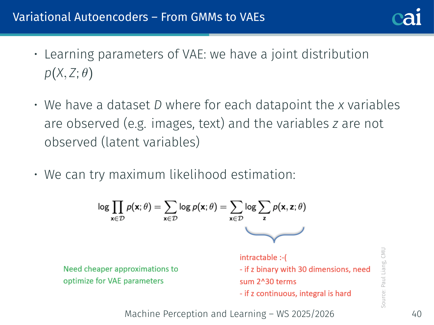
MLE objective on a dataset $\mathcal{D}$:

$\log {\prod }_{x\in \mathcal{D}}p(x;\theta )={\sum }_{x\in \mathcal{D}}\log p(x;\theta )={\sum }_{x\in \mathcal{D}}\log {\sum }_{z}p(x,z;\theta )$

The sum inside the log is intractable for continuous, high-dimensional $z$ — we need a smarter approach.

---

Evidence Lower Bound (ELBO)

Derivation via Jensen’s Inequality

Using Jensen's inequality to derive the ELBO.

Walking through the math to show how ELBO bounds our log-likelihood.

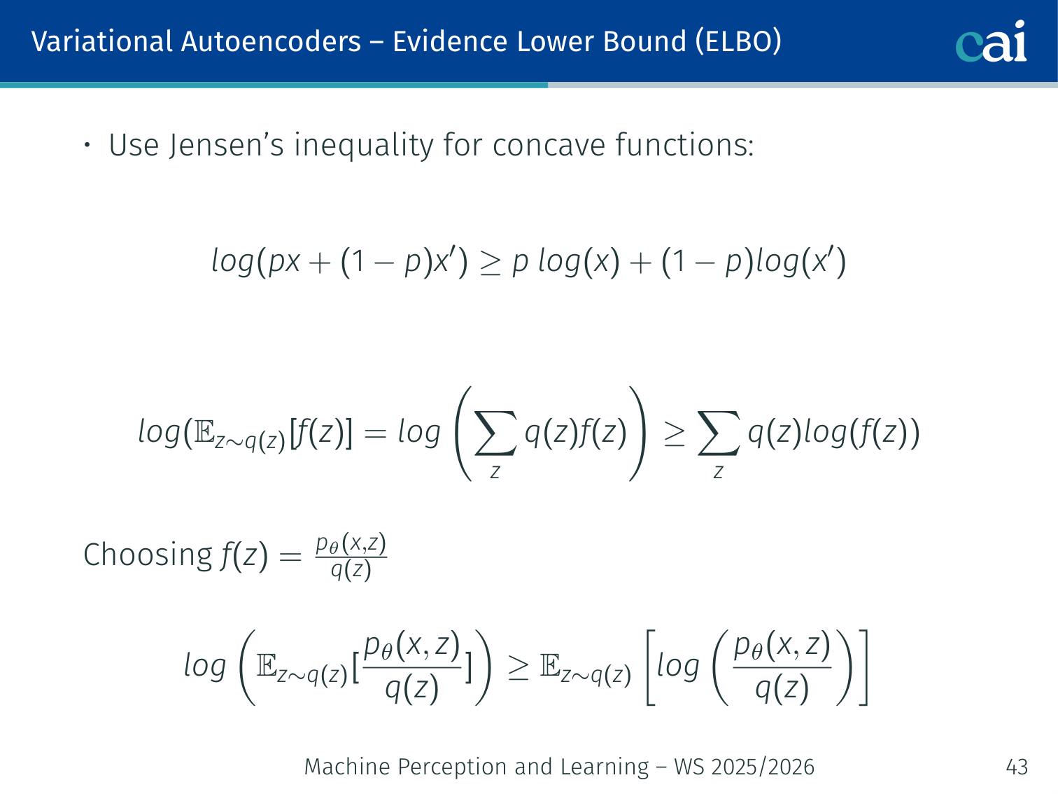
The log-likelihood with latent variables is hard:

$\log p(x;\theta )=\log {\sum }_{z}p(x,z;\theta )=\log {\sum }_z\frac{q(z)}{q(z)}p(x,z;\theta )=\log {\mathbb{E}}_{z\sim q(z)}\left[\frac{p_{\theta }(x,z)}{q(z)}\right]$

where $q(z)$ is any distribution we choose (it should be simple and tractable).

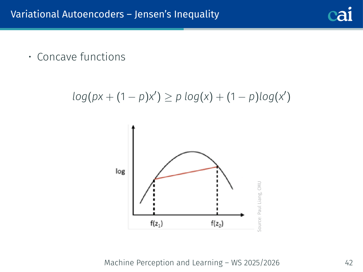
Since $\log$ is concave, Jensen’s inequality gives:

$\log {\mathbb{E}}_{z\sim q}\left[f(z)\right]\ge {\mathbb{E}}_{z\sim q}\left[\log f(z)\right]$

Applying this with $f(z)=p_{\theta }(x,z)/q(z)$:

$\log p(x;\theta )\ge {\mathbb{E}}_{z\sim q(z)}\left[\log \frac{p_{\theta }(x,z)}{q(z)}\right]=:\mathcal{L}(x;\theta ,\varphi )\text{(ELBO)}$

💡 Intuition: What Jensen’s Inequality Is Buying Us

The hard quantity is

$\log \int p_{\theta }(x,z)dz$

because the log of a sum / integral is awkward to optimize directly.

Jensen’s inequality gives us a workaround:

• replace the hard exact objective with something we can actually compute
• make that surrogate objective a lower bound
• tighten the bound by choosing a good approximate posterior $q_{\varphi }(z|x)$

So the ELBO is not a random trick. It is the price we pay for turning an intractable marginal likelihood problem into a tractable optimization problem.

Derivation via KL Divergence

Another way to get the ELBO: using KL divergence between our posteriors.

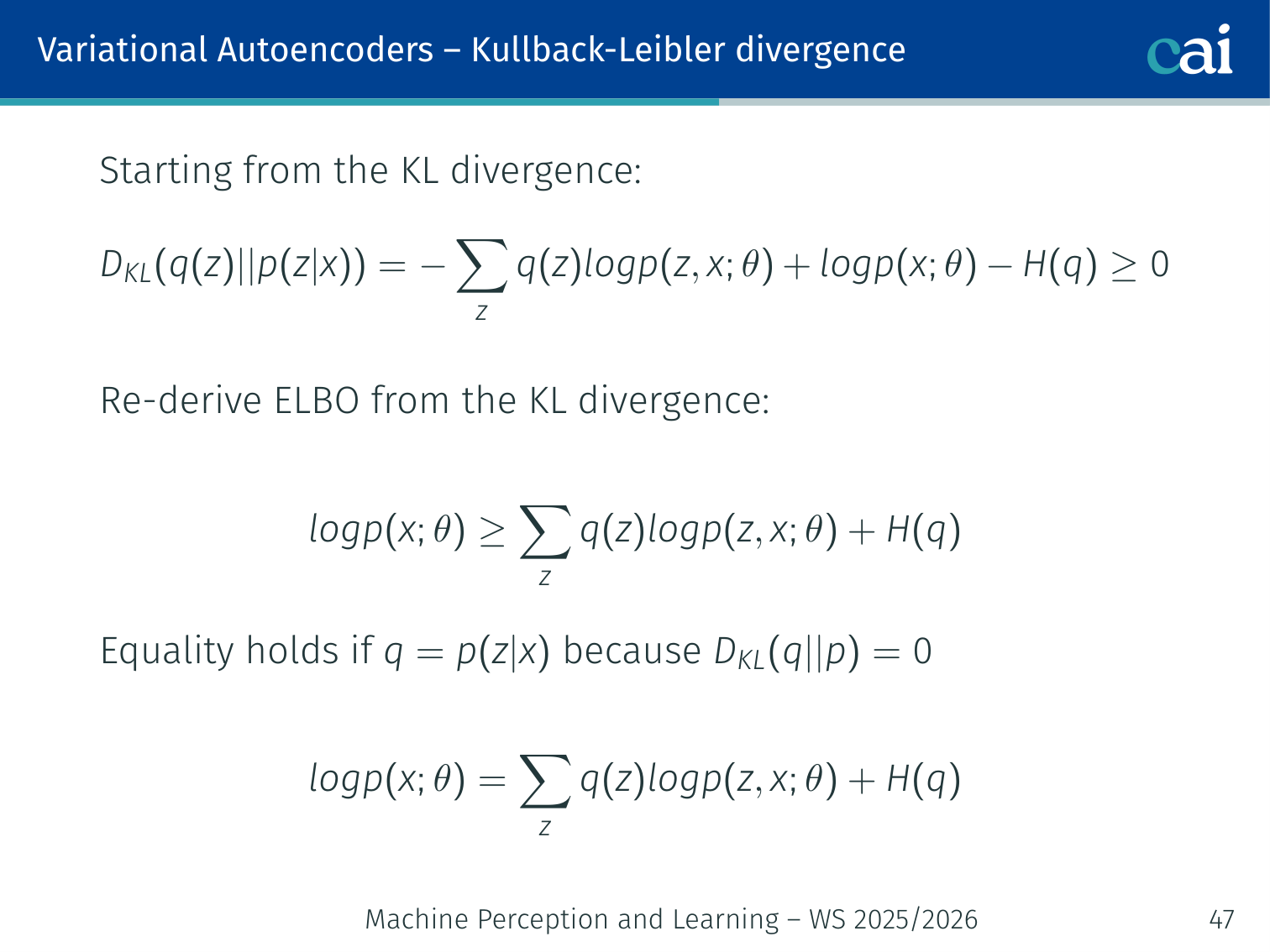
Starting from:

$D_{KL}(q(z)\Vert p(z|x;\theta ))=-{\sum }_{z}q(z)\log p(z,x;\theta )+\log p(x;\theta )-H(q)\ge 0$

Rearranging:

$\log p(x;\theta )\ge \underset{\text{ELBO}}{\underbrace{\sum _{z}q(z)\log p(z,x;\theta )+H(q)}}=\mathcal{L}$

Equality holds when $q=p(z|x)$ because $D_{KL}=0$ in that case.

In general:

$\boxed{\log p(x;\theta )=\mathcal{L}(x;\theta ,\varphi )+D_{KL}(q(z)\Vert p(z|x;\theta ))}$

The closer our chosen $q$ is to the true posterior $p(z|x)$, the tighter the ELBO is to the true likelihood.

ELBO as Reconstruction + KL

Breaking down the ELBO into reconstruction loss and KL regularization.

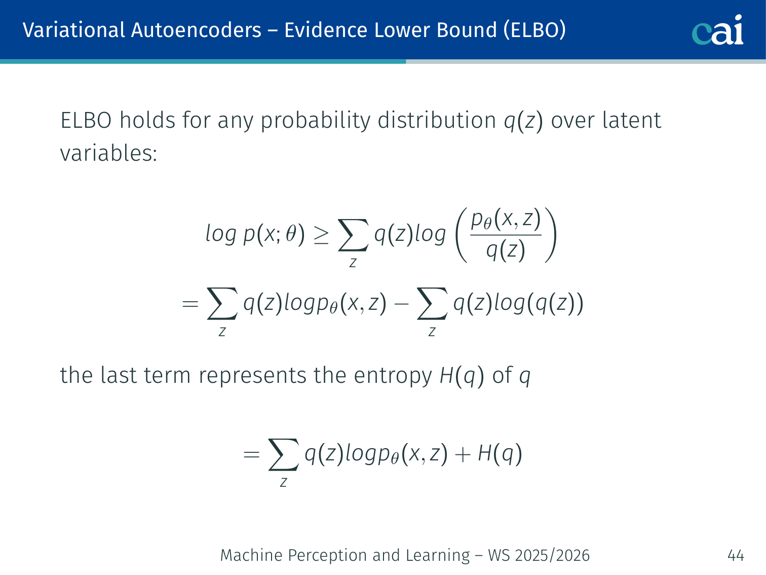
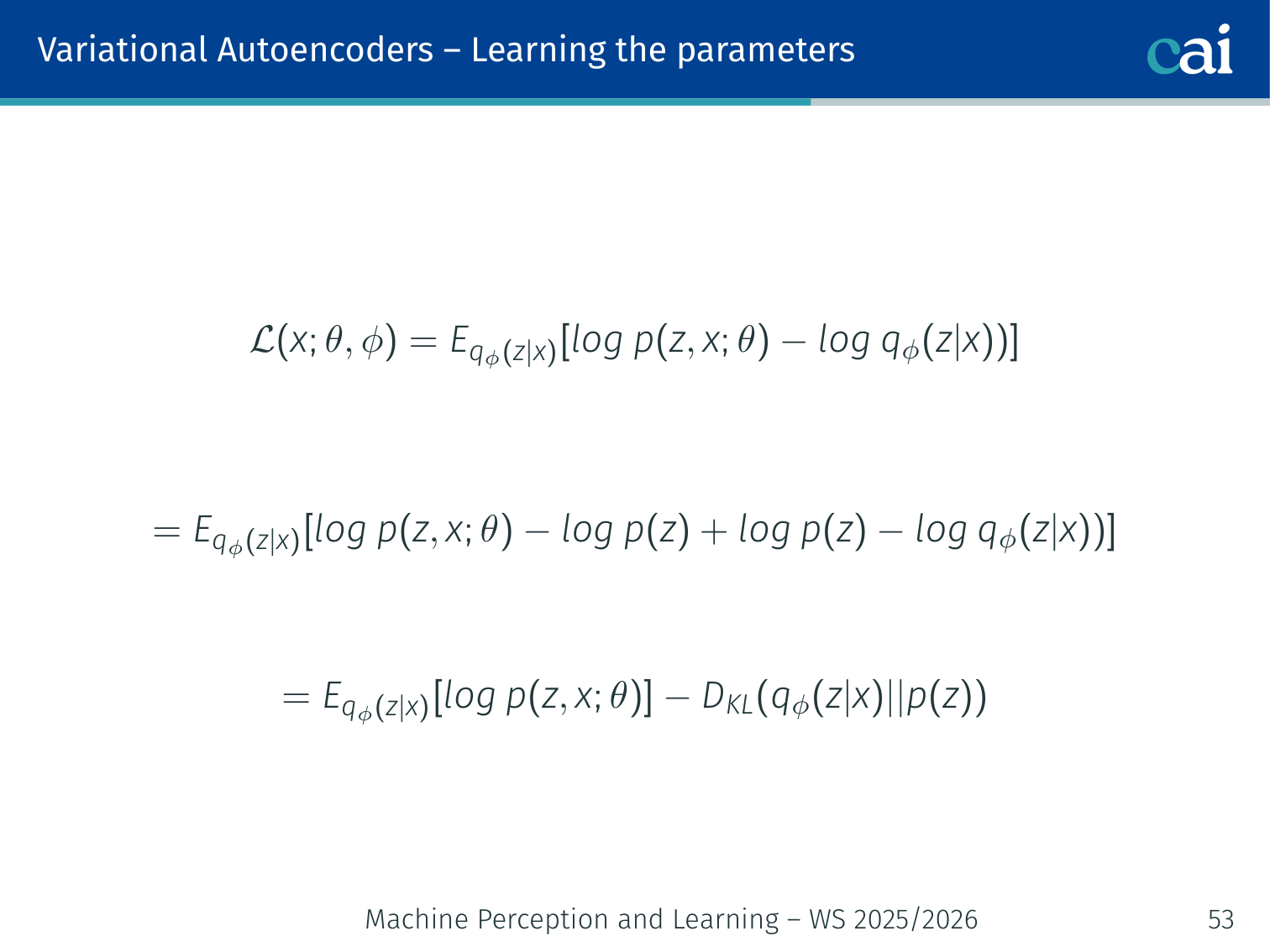
Expanding the ELBO with $q_{\varphi }(z|x)$ as the encoder:

$\mathcal{L}(x;\theta ,\varphi )={\mathbb{E}}_{q_{\varphi }(z|x)}[\log p_{\theta }(x,z)-\log q_{\varphi }(z|x)]$

$={\mathbb{E}}_{q_{\varphi }(z|x)}[\log p_{\theta }(x|z)]-D_{KL}(q_{\varphi }(z|x)\Vert p(z))$

$=\underset{\text{Reconstruction}}{\underbrace{{\mathbb{E}}_{q(z|x)}[\log p_{\theta }(x|z)]}}-\underset{\text{Regularisation}}{\underbrace{D_{KL}(q_{\varphi }(z|x)\Vert p(z))}}$

Term 1 — Reconstruction loss: how well does the decoder recover $x$ from $z$?

• Continuous data ($x\in {\mathbb{R}}^d$): $\Vert x-\hat{x}{\Vert }^2$ (MSE / Gaussian likelihood)
• Binary data (e.g. binarised MNIST): binary cross-entropy

Term 2 — KL divergence: how far is the posterior from the prior $\mathcal{N}(0,I)$?

For Gaussians ($q_{\varphi }(z|x)=\mathcal{N}(\mu ,{\sigma }^{2}I)$, $p(z)=\mathcal{N}(0,I)$) this is analytic:

$D_{KL}=-\frac{1}{2}{\sum }_{j=1}^d\left(1+\log {\sigma }_j^2-{\mu }_j^2-{\sigma }_j^2\right)$

Intuition: The KL term acts as a regularizer pushing each $z_j$ dimension toward $\mathcal{N}(0,1)$. Without it, the encoder can “cheat” by mapping every input to a very narrow distribution (basically the non-generative autoencoder), defeating the purpose.

💡 Intuition: The ELBO Is a Negotiation Between Two Goals

It helps to read the ELBO as a tug-of-war:

• Reconstruction term: “keep enough information in $z$ so the decoder can rebuild the input”
• KL term: “don’t let each datapoint hide in its own weird corner of latent space”

If reconstruction dominates, the model memorizes too much and generation becomes poor. If KL dominates, all posteriors collapse toward the prior and the decoder loses useful information.

VAE training works when these two pressures balance: compress, but not so aggressively that the latent code becomes useless; regularize, but not so strongly that every input looks the same.

---

Variational Inference

Fitting a simple distribution q to a messy, intractable posterior.

We introduce an approximate posterior $q_{\varphi }(z|x)$ (the encoder) — a tractable distribution parametrised by $\varphi$, e.g. a diagonal Gaussian:

$q_{\varphi }(z|x)=\mathcal{N}({\varphi }_1(x),{\varphi }_2(x))$

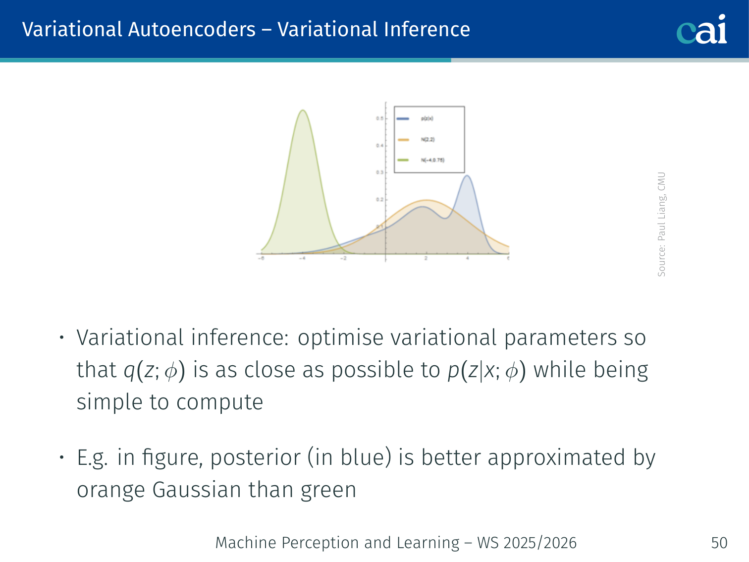
Variational inference: optimise $\varphi$ so that $q_{\varphi }(z|x)$ is as close as possible to the true posterior $p(z|x;\theta )$, while remaining simple to compute.

Example: the true posterior $p(z|x)$ (shown in blue) might be a skewed non-Gaussian shape. The variational distribution $q_{\varphi }$ (a Gaussian, shown in orange) is fit to approximate it. A poor choice (green) fails to capture the posterior’s mass.

The key insight of VAEs is to amortise this inference: instead of running optimisation at test time for every $x$, train an encoder network $E_{\varphi }$ that directly maps $x\to ({\mu }_{\varphi },{\sigma }_{\varphi })$ in a single forward pass.

---

Learning the Parameters

Training a VAE by optimizing the encoder and decoder together through the ELBO.

We jointly optimise decoder parameters $\theta$ and encoder parameters $\varphi$ by maximising the ELBO:

$\mathcal{L}(x;\theta ,\varphi )={\mathbb{E}}_{q_{\varphi }(z|x)}[\log p_{\theta }(x|z)]-D_{KL}(q_{\varphi }(z|x)\Vert p(z))$

Gradient w.r.t. $\theta$ (decoder — straightforward):

${\nabla }_{\theta }\mathcal{L}={\nabla }_{\theta }{\mathbb{E}}_{q_{\varphi }(z|x)}[\log p_{\theta }(x|z)]={\mathbb{E}}_{q_{\varphi }(z|x)}[{\nabla }_{\theta }\log p_{\theta }(x|z)]\approx \frac{1}{n}{\sum }_{i=1}^n{\nabla }_{\theta }\log p_{\theta }(x|z_i;\theta )$

Since $\theta$ does not appear inside the expectation distribution, we can move the gradient inside freely.

Gradient w.r.t. $\varphi$ (encoder — tricky):

${\nabla }_{\varphi }\mathcal{L}={\nabla }_{\varphi }{\mathbb{E}}_{q_{\varphi }(z|x)}[\log p_{\theta }(x|z)]-{\nabla }_{\varphi }{D}_{KL}$

The expectation itself depends on $\varphi$ (it is the distribution we sample $z$ from), so we cannot naively move ${\nabla }_{\varphi }$ inside. This requires the reparameterization trick.

---

The Reparameterization Trick

Problem: $z\sim q_{\varphi }(z|x)$ is a stochastic sampling step — gradients cannot flow through it.

Solution: express the sample as a deterministic function of $(\varphi ,\epsilon )$ where $\epsilon$ is noise that doesn’t depend on the parameters:

$z={\mu }_{\varphi }(x)+{\sigma }_{\varphi }(x)\odot \epsilon ,\epsilon \sim \mathcal{N}(0,I)$

Now the expectation becomes:

${\mathbb{E}}_{z\sim q_{\varphi }}[r(z)]={\mathbb{E}}_{\epsilon \sim \mathcal{N}(0,I)}[r(\mu +\sigma \epsilon )]$

And the gradient moves inside cleanly:

${\nabla }_{\varphi }{\mathbb{E}}_{q_{\varphi }}[r(z)]={\mathbb{E}}_{\epsilon }[{\nabla }_{\varphi }r(\mu +\sigma \epsilon )]\approx \frac{1}{n}{\sum }_{i=1}^n{\nabla }_{\varphi }r(\mu +\sigma {\epsilon }_i)$

The randomness ($\epsilon$) is now external — gradients flow back through ${\mu }_{\varphi }$ and ${\sigma }_{\varphi }$ via standard backpropagation.

🧠 Deep Dive: Why Sampling Breaks Backprop

Backprop needs each operation to be a differentiable function of the parameters.

If we write only

$z\sim q_{\varphi }(z|x)$

then the computational graph has a “gap”: the sampled value $z$ changes when $\varphi$ changes, but not through an explicit differentiable formula that autograd can trace.

The reparameterization trick repairs that gap by rewriting sampling as:

1. draw noise $\epsilon \sim \mathcal{N}(0,I)$ from a fixed distribution
2. transform it deterministically using ${\mu }_{\varphi }(x)$ and ${\sigma }_{\varphi }(x)$

That is exactly the move used in the original AEVB paper: push the randomness into an auxiliary variable that does not depend on the learnable parameters, so gradient-based optimization becomes straightforward.

              ε ~ N(0,I)   ← external noise, no gradient
                  │
x ──→ Encoder ──→ μ, σ
                  │  z = μ + σ⊙ε
                  ↓
               Decoder ──→ x̂
                  ↓
               ELBO loss

Example: without reparameterization, training a VAE on MNIST wouldn’t converge — the KL term would not receive gradients back to the encoder. With reparameterization, the encoder learns to produce posteriors that both reconstruct well and stay close to $\mathcal{N}(0,I)$.

---

Generating Data

At training time: requires both encoder and decoder (compute ELBO).

At inference / generation time: only the decoder is needed.

1. Sample $z\sim p(z)=\mathcal{N}(0,I)$
2. Pass through decoder: $\hat{x}=g_{\theta }(z)$

The KL regularization ensures this works — because the encoder is trained to push $q_{\varphi }(z|x)\approx \mathcal{N}(0,I)$, any random $z$ from the prior decodes to a plausible image.

💡 Intuition: Why Sampling From the Prior Works at All

The whole point of the KL term is to make the encoder’s posterior clouds live in roughly the same region as the simple prior.

So generation works because training tries to align two things:

• where real datapoints get encoded
• where random latent samples come from

If those two regions overlap well, then drawing

$z\sim \mathcal{N}(0,I)$

lands you in territory the decoder has effectively been trained to understand.

---

Latent Space Properties

Because the KL term regularizes $z$ toward $\mathcal{N}(0,I)$, the latent space has structure:

1. Continuity: nearby points in $z$ decode to visually similar outputs
2. Completeness: any $z\sim \mathcal{N}(0,I)$ decodes to something valid
3. Smooth interpolation: linearly interpolating between two $z$ codes gives a smooth visual transition

Example: Face Interpolation

α = 0.0       α = 0.25      α = 0.50      α = 0.75      α = 1.0
z_A ──────────────────────────────────────────────────────→ z_B
[face A] → [blend 25%] → [blend 50%] → [blend 75%] → [face B]

With a standard autoencoder, decoding points between $z_A$ and $z_B$ would give noise. With a VAE, you get a smooth morphing sequence.

💡 Intuition: Why Interpolation Is a Better Test Than Reconstruction

Reconstruction only asks: “can the model copy training-like examples?”

Interpolation asks something deeper:

• does the latent space contain meaningful paths between examples?
• do intermediate points still decode to valid data?

That is why interpolation is such a good sanity check for VAEs. If the path between two encoded samples stays on the data manifold, the latent space is doing something genuinely useful rather than just memorizing isolated points.

Latent Space Arithmetic

Semantic arithmetic: doing math in the latent space to transform images.

Like word2vec arithmetic (king − man + woman ≈ queen), VAE latent codes support semantic arithmetic:

z("smiling woman") − z("neutral woman") + z("neutral man") ≈ z("smiling man")

---

Autoencoder vs. VAE Latent Spaces

	Regular Autoencoder	VAE
Encoder output	Single point $z$	Distribution $(\mu ,\sigma )$
Latent space	Irregular, discontinuous	Smooth, structured
Random sampling	Mostly garbage	Valid outputs
Interpolation	Discontinuous	Smooth

MNIST visualisation: a regular AE has tight digit clusters with large empty gaps — random samples from the gaps are meaningless. A VAE has overlapping, smoothly-varying clusters — samples from anywhere produce recognisable (if blurry) digits.

---

Applications

Disentangled Representation Learning

Using beta-VAE to pull apart independent factors of variation.

Entangled vs. disentangled latent spaces for better control.

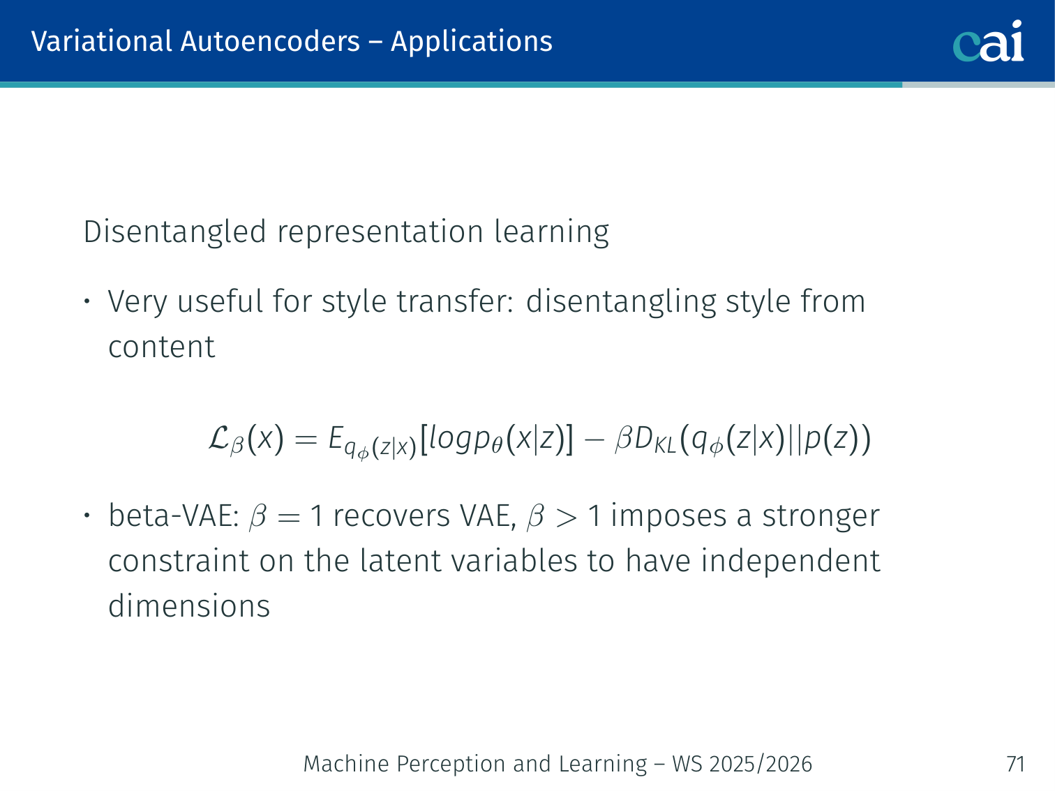
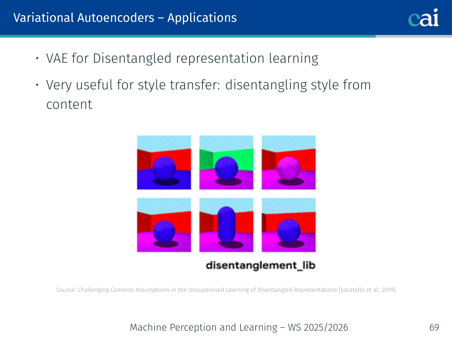
Goal: learn a latent space where each dimension controls an independent, interpretable factor (e.g. one dimension = pose, another = lighting).

The beta-VAE [Higgins et al., 2017] adds a hyperparameter $\beta$ to weight the KL term:

${\mathcal{L}}_{\beta }(x)={\mathbb{E}}_{q_{\varphi }(z|x)}[\log p_{\theta }(x|z)]-\beta D_{KL}(q_{\varphi }(z|x)\Vert p(z))$

• $\beta =1$: recovers the standard VAE
• $\beta >1$: imposes a stronger constraint, encouraging independent latent dimensions (disentanglement) at the cost of reconstruction quality

[Locatello et al., 2019] showed that unsupervised disentanglement is hard without inductive biases — there are many equally valid disentangled representations.

🧠 Deep Dive: What $\beta >1$ Is Really Buying You

The beta-VAE paper frames $\beta$ as a knob that changes the balance between reconstruction fidelity and latent factorization / channel capacity.

• With $\beta =1$, we recover the standard VAE objective.
• With $\beta >1$, the model is penalized more strongly for encoding too much information in a tangled way.

This creates pressure to use the latent dimensions more economically. In the best case, each dimension starts specializing in one interpretable factor such as pose, thickness, rotation, or lighting.

The tradeoff is real, though:

• stronger disentanglement pressure can improve interpretability
• but reconstructions often get worse because the bottleneck becomes harsher

So beta-VAE is not “strictly better VAE.” It is a deliberate trade: less raw fidelity, more structured latents.

Style Transfer (Text and Images)

Using VAEs for style transfer in both images and text.

VAEs disentangle style from content in the latent space. Applications:

• Image style transfer: given content image $x_1$ and style $c$, generate $p(x_2|x_1,c)$. [Gatys et al., 2016]
• Text style transfer: encode a sentence, manipulate the style dimension (e.g. sentiment), decode back. [Shen et al., 2017]

Handwriting Synthesis (Aksan et al., 2018)

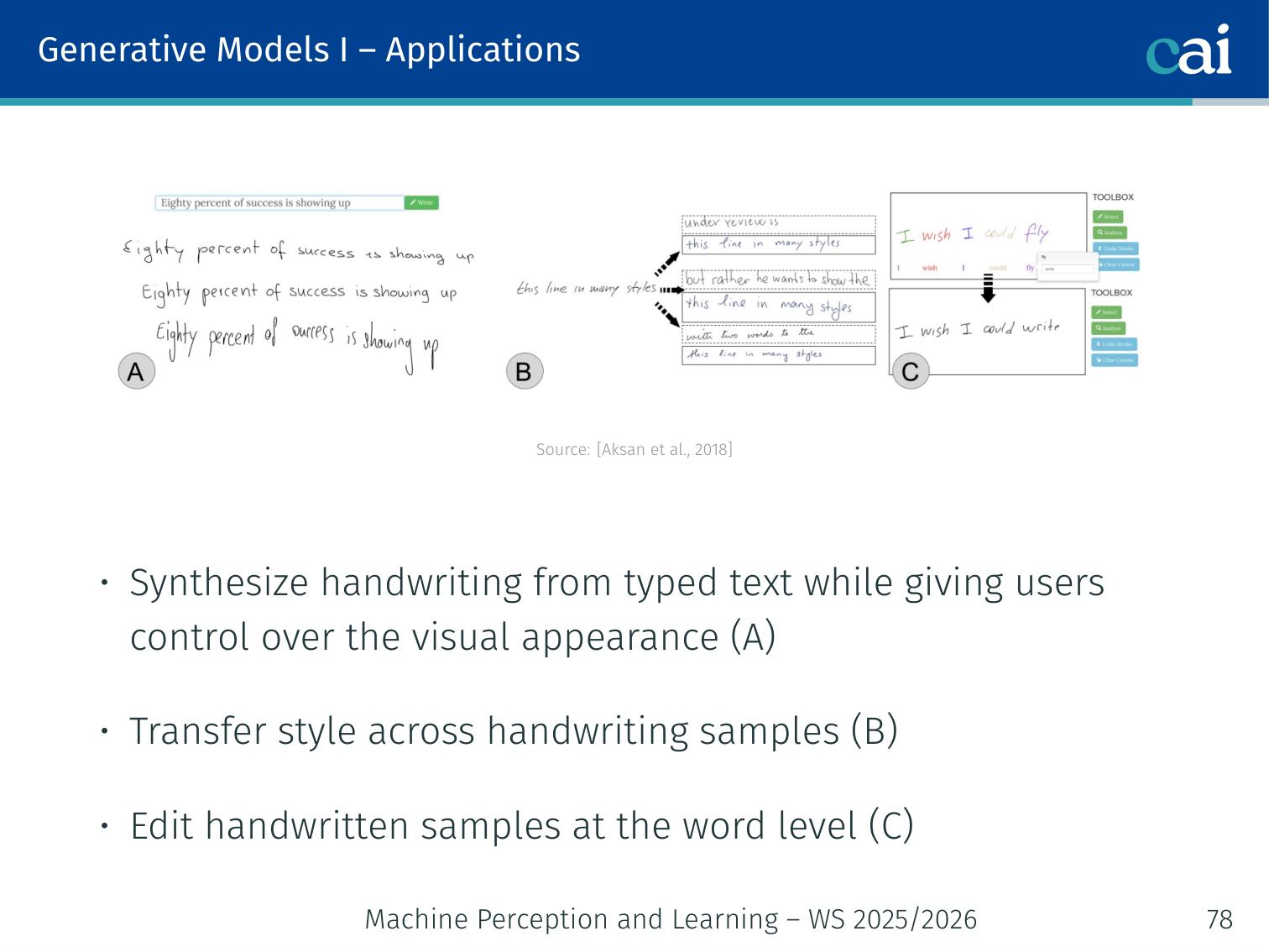
Editing and generating synthetic handwriting on a VAE manifold.

A VAE trained on handwriting samples can:

• (A) Synthesize handwriting from typed text while giving users control over visual appearance (style)
• (B) Transfer style across handwriting samples
• (C) Edit handwritten samples at the word level

Hand Pose Manifold (Tagliasacchi et al., 2015)

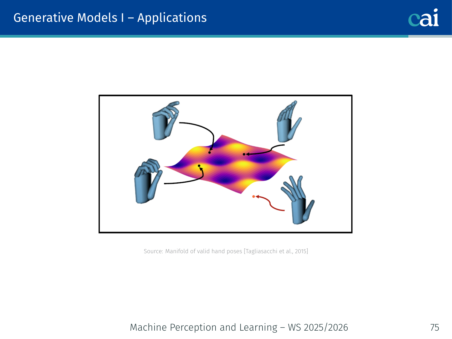
Mapping hand poses to a smooth manifold for better pose estimation.

A VAE trained on hand pose data learns a smooth, compact manifold of valid hand configurations. Sampling from the manifold always produces a valid (anatomically plausible) hand pose — useful for 3D pose estimation from noisy depth sensors.

PyTorch Implementation: Convolutional VAE

Below is a convolutional implementation of a Variational Autoencoder (VAE). This architecture is much more effective than a simple MLP for generating images.

import torch
import torch.nn as nn
import torch.nn.functional as F
 
# 1. The ENCODER: compresses image into (mean, log_variance)
class Encoder(nn.Module):
    def __init__(self, latent_dim):
        super().__init__()
        # Convolutional layers extract hierarchical spatial features
        self.conv1 = nn.Conv2d(1, 6, 5)
        self.conv2 = nn.Conv2d(6, 16, 5)
 
        # Two parallel linear heads: one for mean, one for log-variance
        # These represent the distribution of the latent code 'z'
        self.fc_mu = nn.Linear(16 * 4 * 4, latent_dim)
        self.fc_logvar = nn.Linear(16 * 4 * 4, latent_dim)
 
    def forward(self, x):
        x = F.max_pool2d(F.relu(self.conv1(x)), 2)
        x = F.max_pool2d(F.relu(self.conv2(x)), 2)
        x = x.view(x.size(0), -1) # Flatten for linear layers
        return self.fc_mu(x), self.fc_logvar(x)
 
# 2. The DECODER: reconstructs the image from a latent sample
class Decoder(nn.Module):
    def __init__(self, latent_dim):
        super().__init__()
        self.fc = nn.Linear(latent_dim, 16 * 7 * 7)
        # Transposed convolutions (deconvolutions) upsample the features
        # back to the original image resolution (28x28)
        self.deconv1 = nn.ConvTranspose2d(16, 6, 4, stride=2, padding=1)
        self.deconv2 = nn.ConvTranspose2d(6, 1, 4, stride=2, padding=1)
 
    def forward(self, z):
        x = F.relu(self.fc(z)).view(-1, 16, 7, 7) # Reshape back to 4D
        x = F.relu(self.deconv1(x))
        # Sigmoid ensures output pixels are in range [0, 1]
        return torch.sigmoid(self.deconv2(x))
 
# 3. The VAE WRAPPER: combines encoder, decoder, and sampling trick
class VAE(nn.Module):
    def __init__(self, latent_dim=20):
        super().__init__()
        self.encoder = Encoder(latent_dim)
        self.decoder = Decoder(latent_dim)
 
    def reparameterize(self, mu, logvar):
        """
        The Reparameterization Trick:
        Sample z = mu + std * epsilon, where epsilon is random noise.
        This allows gradients to flow back through the mu and logvar heads.
        """
        std = torch.exp(0.5 * logvar)
        eps = torch.randn_like(std)
        return mu + eps * std
 
    def forward(self, x):
        # 1. Get distribution parameters from image
        mu, logvar = self.encoder(x)
        # 2. Sample a code 'z' from that distribution
        z = self.reparameterize(mu, logvar)
        # 3. Reconstruct image from the sample
        return self.decoder(z), mu, logvar

Key VAE Concepts:

• The Sampling Trick: By sampling z this way, the randomness is externalized. During the backward pass, PyTorch can differentiate through the mu and logvar parameters.
• Latent Space Continuity: The KL-divergence loss (used in training) forces the z codes to cluster around $\mathcal{N}(0,1)$. This ensures there are no large “gaps” in the latent space, making it easy to sample new, valid images.
• Transposed Convolution: Unlike normal convolution that reduces resolution, ConvTranspose2d learns how to fill in pixels to increase the image size.

---

Summary of VAEs

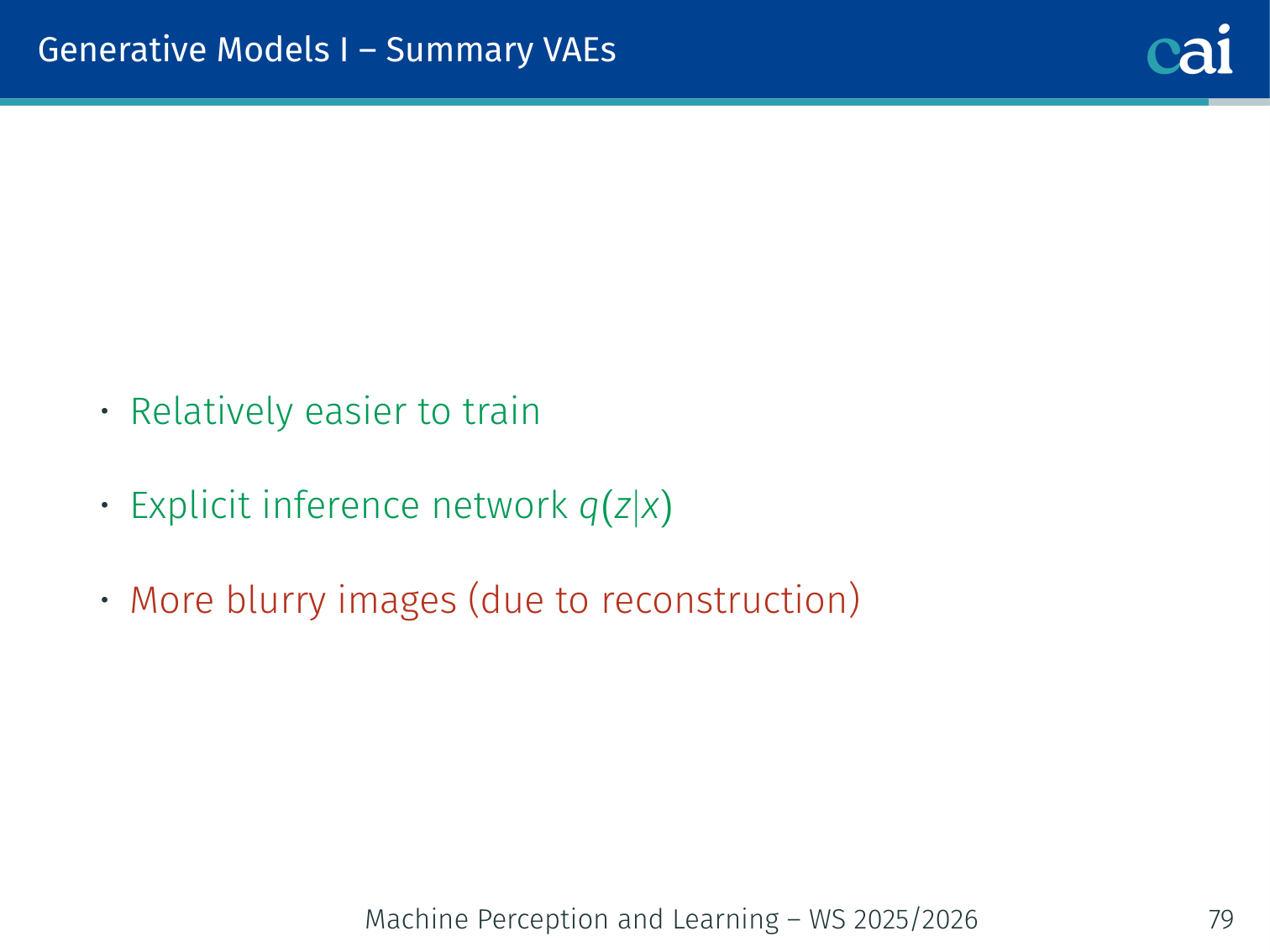
A wrap-up of VAEs: they're principled and smooth, but can be a bit blurry.

Aspect	Detail
Pros	Relatively easy to train; explicit inference network $q(z\mid x)$; principled probabilistic framework; smooth latent space
Cons	Blurry samples (MSE averages over uncertainty); ELBO is a lower bound (no exact likelihood)
vs. AE	Adds KL regularization → structured, sampleable latent space
vs. GAN	More stable training; explicit likelihood; but lower sharpness
vs. Diffusion	Faster sampling; but lower sample quality

Why blurry? Optimizing MSE reconstruction encourages the decoder to output the mean of all possible reconstructions consistent with $z$, rather than a single sharp sample. This is the classic regression-to-the-mean problem.

---

VAEs vs. Other Generative Models

Model	Latent Space	Sample Quality	Training Stability
Autoencoder	Unstructured	Bad (gap problem)	Stable
VAE	Structured, continuous	OK (blurry)	Stable
GAN	Implicit	Sharp, high quality	Unstable (mode collapse)
Diffusion	Hierarchical noise	Excellent	Stable

Applied Exam Focus

• Reparameterization Trick: Instead of sampling $z\sim \mathcal{N}(\mu ,{\sigma }^2)$ directly (which is non-differentiable), sample $ϵ\sim \mathcal{N}(0,1)$ and compute $z=\mu +\sigma \odot ϵ$. This allows Backprop to work.
• Latent Space: The KL-Divergence term in the loss forces the latent space to be a smooth, continuous Gaussian, enabling meaningful interpolation.
• ELBO: The Evidence Lower Bound is the training objective that balances reconstruction quality with latent space regularity.

---

Previous: L08 — IML | Back to MPL Index | Next: (y-10) GANs | (y) Return to Notes | (y) Return to Home