L10 — Generative Adversarial Networks (GANs)

Previous: L09 — VAE | Back to MPL Index | Next: (y-11) RL

University of Stuttgart — Machine Perception and Learning for Collaborative Intelligent Systems, Prof. Dr. Andreas Bulling, WS 2025/2026

---

Mental Model First

• GANs learn to generate data through a game between a generator and a discriminator.
• The discriminator acts like a learned training signal for realism, which is why GANs can produce very sharp samples.
• The hard part is optimization: two networks are changing at once, so stability matters as much as model capacity.
• If one question guides this lecture, let it be: how can a model learn to sample realistic data without ever writing down an explicit density?

VAE Recap

A quick recap of VAEs and their probabilistic bits.

• VAEs are a probabilistic version of autoencoders that allow sampling to generate new, unseen samples.
• A prior is placed on the latent code: $z\sim \mathcal{N}(0,I)$
• The decoder learns $p(x|z)=\mathcal{N}({\mu }_{\theta }(z),{\Sigma }_{\theta }(z))$ where ${\mu }_{\theta }$ and ${\Sigma }_{\theta }$ are neural networks.
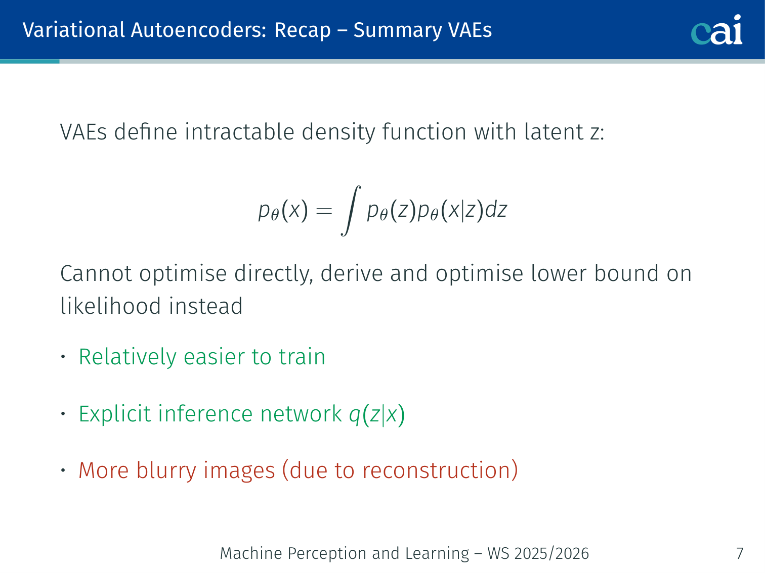
• The intractable density is:

$p_{\theta }(x)=\int p_{\theta }(z)p_{\theta }(x|z)dz$

• Since this can’t be optimised directly, we derive and optimise a lower bound (ELBO) on the likelihood.

Summary of VAEs

A summary of VAEs: easy to train, but there's a tradeoff with image quality.

Property	VAE
Training	Relatively easier
Inference	Explicit inference network $q(z\mid x)$
Image quality	More blurry (due to reconstruction loss)
Density	Explicit but intractable

---

Motivation: From Explicit to Implicit Density

Why we're moving from explicit density models to implicit sampling with GANs.

What if we give up on explicitly modelling the density, and just want the ability to sample?

High-dimensional $p(x)$ is:

• Difficult to evaluate and optimise
• A high $p(x)$ may not correspond to visually realistic samples

This motivates implicit density models — we don’t write down $p(x)$ at all. We only care about samples.

The Two-Sample Test Intuition

The two-sample test: can you tell the real samples from the generated ones?

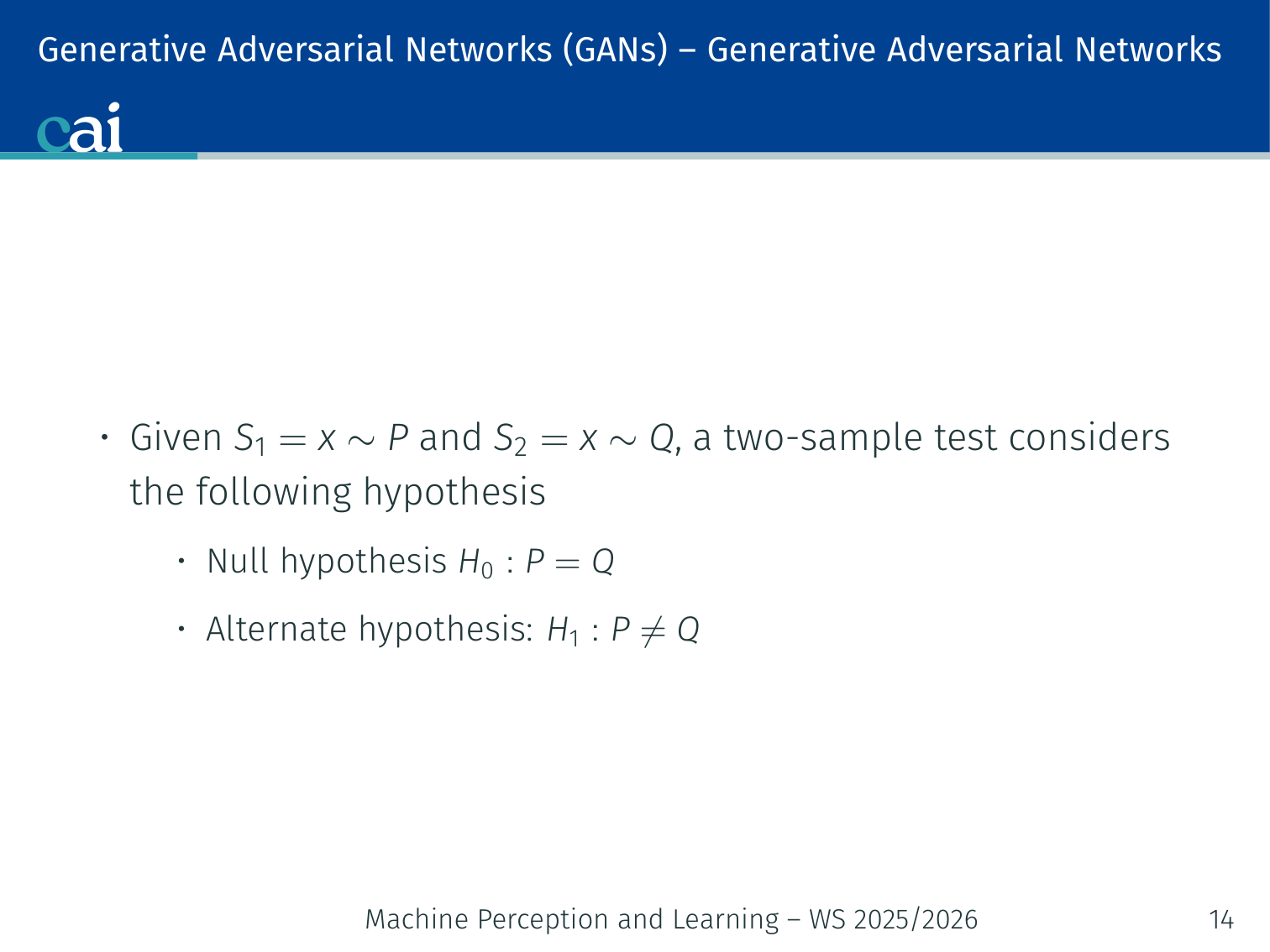
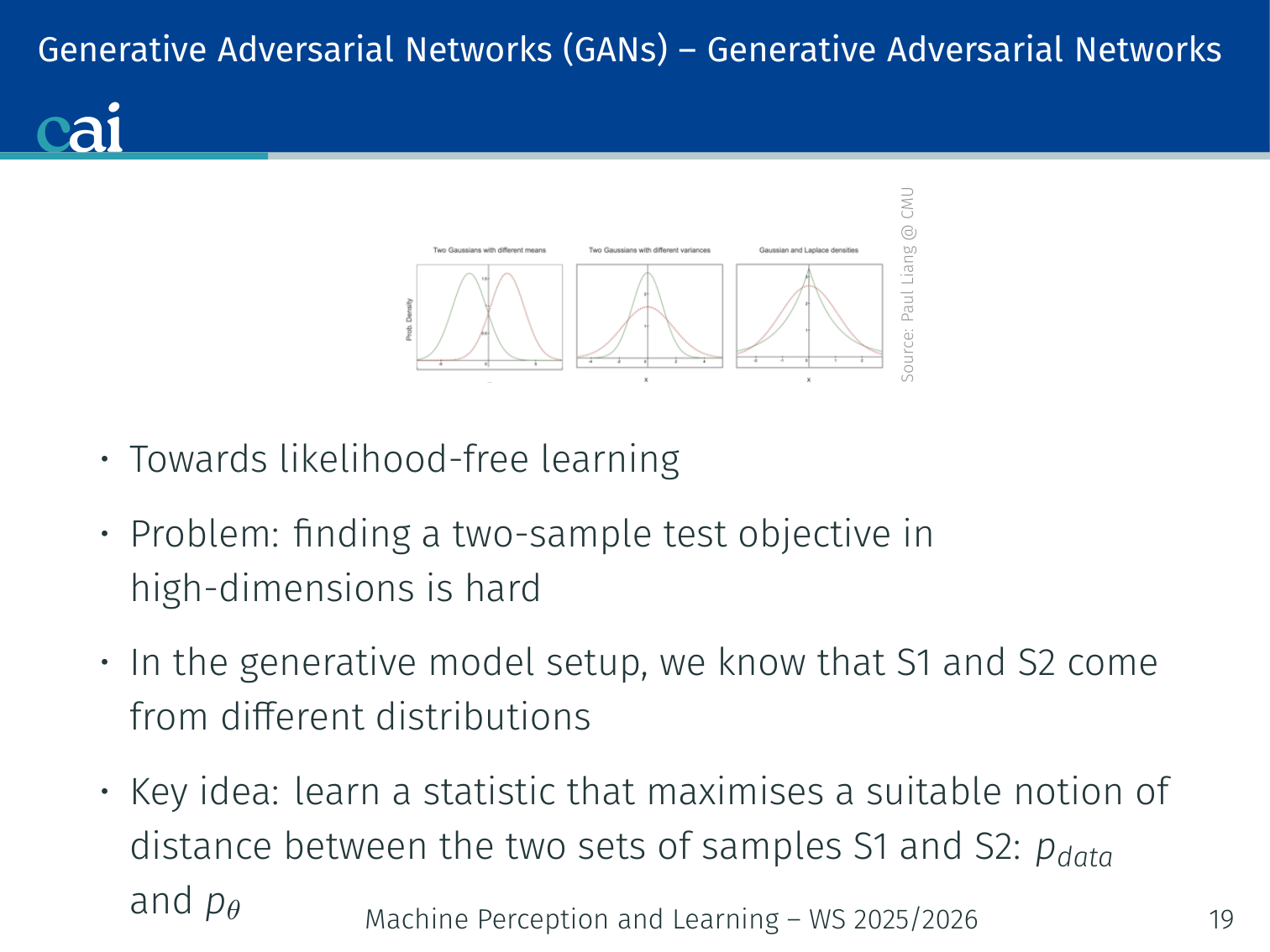
The core question GANs are built on: Given two finite sets of samples, how can we tell if they come from the same distribution?

• $S_1=\{x\sim p_{data}\}$ — real data
• $S_2=\{x\sim p_{\theta }\}$ — model samples

We set up a hypothesis test:

• Null hypothesis $H_0$: $P=Q$ (distributions are the same)
• Alternate hypothesis $H_1$: $P\ne Q$

The test statistic $T$ compares $S_1$ and $S_2$ in terms of means and variance. If $T<\alpha$, we accept $H_0$.

Key observation: The test statistic is likelihood-free — it only uses samples, not the densities $P$ or $Q$ directly.

The GAN Idea

The core of GANs: learning to transform noise z into data samples x.

Instead of hand-designing a test statistic, learn one:

Train the generative model to minimise a two-sample test objective between $S_1=p_{data}$ and $S_2=p_{\theta }$.

Finding a two-sample test objective in high dimensions is hard, so we:

1. Sample from a simple distribution $z\sim p_z$ (e.g., Gaussian noise)
2. Learn a transformation $G:z\mapsto x$ using a neural network
3. Use another neural network to learn the test statistic

---

💡 Intuition: The Counterfeiter and the Detective

The GAN is a two-player game between:

• The Generator (The Counterfeiter): Their goal is to create fake banknotes that are so good, nobody can tell they aren’t real. They never see real money; they only hear from the detective whether their latest batch was caught.
• The Discriminator (The Detective): Their goal is to look at a banknote and decide if it’s real or fake. They study real money to learn what it looks like, and then try to catch the counterfeiter.

As the detective gets better at spotting flaws, the counterfeiter is forced to fix those specific flaws. Eventually, the fakes become indistinguishable from the real thing.

---

🧠 Deep Dive: Mode Collapse (The “Easy Way Out”)

Imagine the counterfeiter discovers that the detective is currently very bad at spotting fake €10 bills, but very good at spotting €50 bills.

Instead of trying to learn how to make all types of money, the counterfeiter might decide to only make €10 bills. Even if they produce millions of identical €10 bills, they are “winning” the game because the detective is fooled.

In Machine Learning: A GAN trained on cats and dogs might “collapse” and only produce one specific, high-quality image of a cat. It has “solved” the problem of fooling the discriminator, but it has failed at its true goal: learning the full diversity of the data distribution.

---

The Adversarial Framework

The GAN architecture: a generator and a discriminator in a constant battle.

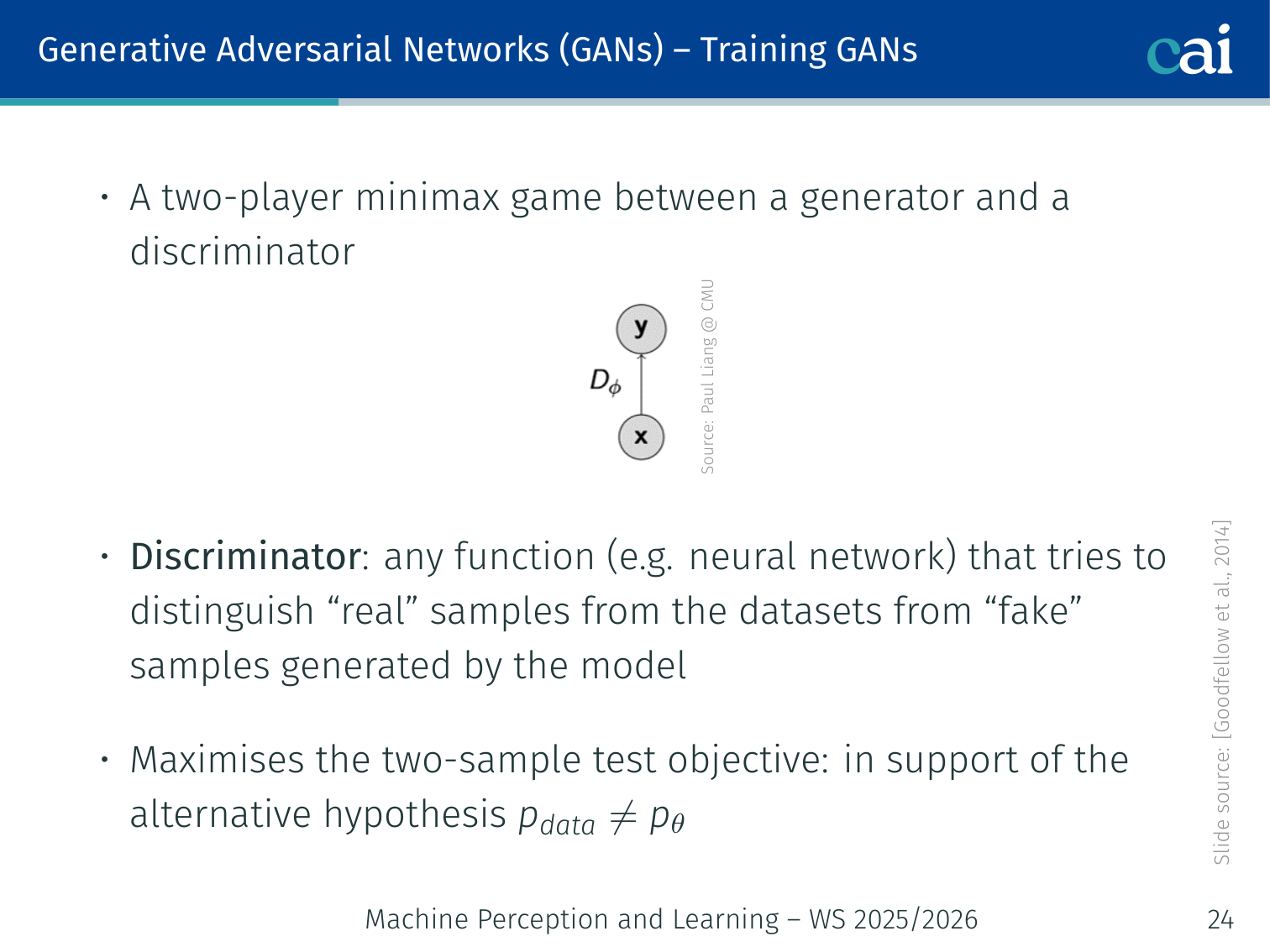
Two neural networks compete in a minimax game (Goodfellow et al., 2014):

Network	Role	Goal
Generator $G$	Transforms noise $z\sim p_z$ into fake samples	Fool the discriminator — support $H_0:p_{data}=p_{\theta }$
Discriminator $D$	Classifies real vs. fake samples	Distinguish — support $H_1:p_{data}\ne p_{\theta }$

Noise z ~ p_z ──→ [Generator G] ──→ fake x̂
                                          │
Real data x ~ p_data ──────────────→ [Discriminator D] ──→ Real (1) / Fake (0)

The generator never sees real data directly — it only receives feedback through the discriminator’s gradient.

Example intuition — a counterfeiter and a police detective:

• The counterfeiter (G) makes fake banknotes and tries to pass them off as real.
• The detective (D) examines banknotes and tries to identify fakes.
• As the detective gets better, the counterfeiter is forced to improve. Eventually, the fakes become indistinguishable from real notes.

---

Training Objectives

Discriminator Objective

The discriminator's goal: get as good as possible at spotting real vs. fake data.

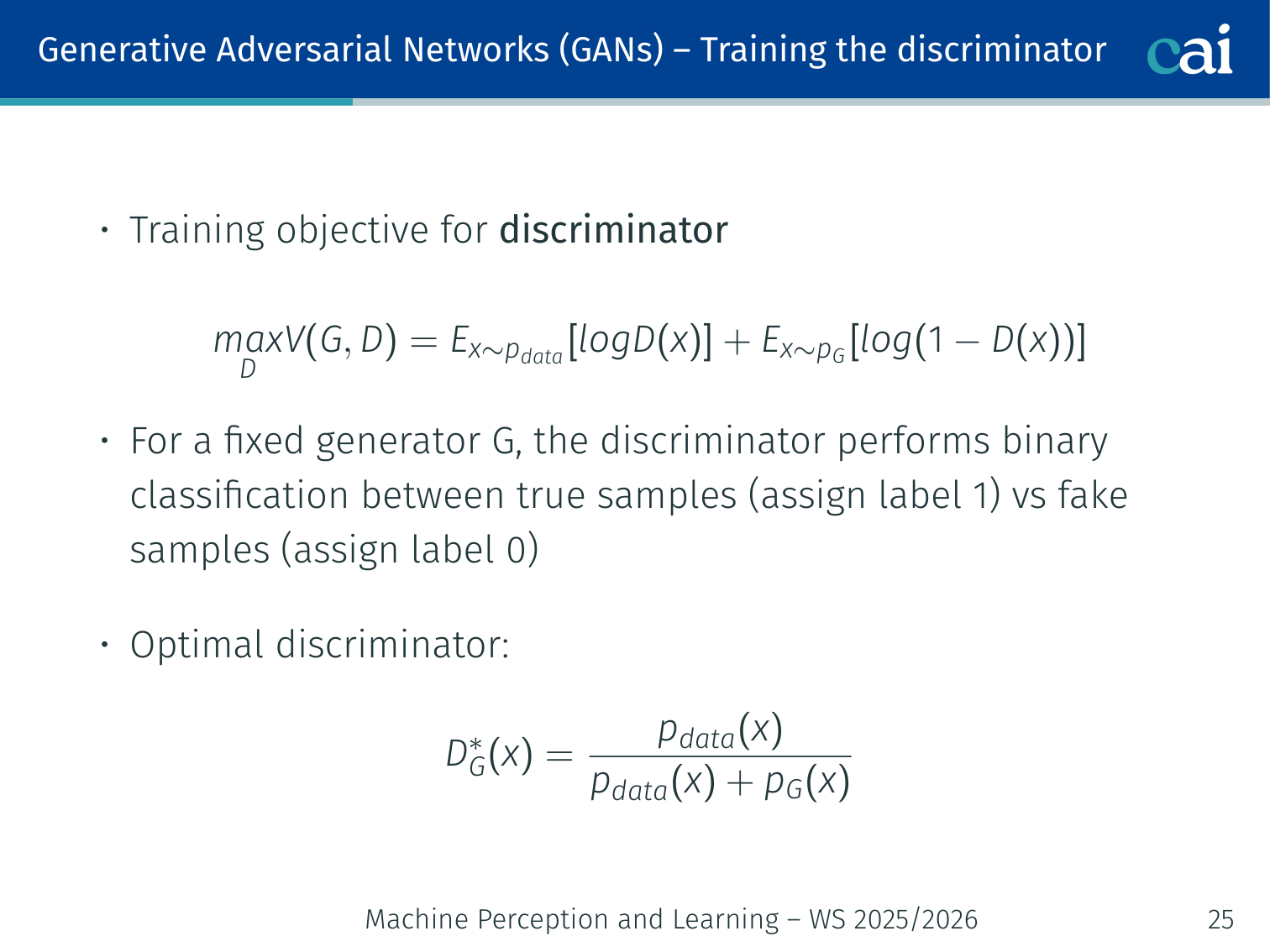
The discriminator performs binary classification — real samples get label 1, fake samples get label 0:

${\max }_{D}V(G,D)={\mathbb{E}}_{x\sim p_{data}}[\log D(x)]+{\mathbb{E}}_{x\sim p_G}[\log (1-D(x))]$

This is a standard binary cross-entropy loss. For a fixed generator $G$, the optimal discriminator is:

$D_G^{\ast }(x)=\frac{p_{data}(x)}{p_{data}(x)+p_G(x)}$

Example: if at a given point $x$, half the density is real and half is fake, the optimal discriminator outputs $D^{\ast }(x)=0.5$ — it cannot do better than chance there.

Generator Objective

The generator minimises the same quantity — it wants the discriminator to fail:

${\min }_{G}V(G,D)={\mathbb{E}}_{x\sim p_{data}}[\log D(x)]+{\mathbb{E}}_{x\sim p_G}[\log (1-D(x))]$

Combined Minimax Objective

${\min }_G{\max }_D\mathcal{L}(D,G)={\mathbb{E}}_{x\sim p_{data}}[\log D(x)]+{\mathbb{E}}_{z\sim p_z}[\log (1-D(G(z)))]$

Connection to Jensen-Shannon Divergence

Substituting the optimal discriminator $D_G^{\ast }$ into the objective:

$V(G,D_G^{\ast })={\mathbb{E}}_{x\sim p_{data}}\left[\log \frac{p_{data}(x)}{p_{data}(x)+p_G(x)}\right]+{\mathbb{E}}_{x\sim p_G}\left[\log \frac{p_G(x)}{p_{data}(x)+p_G(x)}\right]$

$=D_{KL}\left[p_{data},\frac{p_{data}+p_G}{2}\right]+D_{KL}\left[p_G,\frac{p_{data}+p_G}{2}\right]-\log 4$

$=2D_{JSD}[p_{data},p_G]-\log 4$

So the vanilla GAN objective is equivalent to minimising the Jensen-Shannon Divergence between the data and generator distributions.

The Jensen-Shannon Divergence (also called symmetric KL):

$D_{JSD}=\frac{1}{2}\left(D_{KL}\left[p,\frac{p+q}{2}\right]+D_{KL}\left[q,\frac{p+q}{2}\right]\right)$

Properties:

• $D_{JSD}[p,q]\ge 0$
• $D_{JSD}[p,q]=0⟺p=q$
• $D_{JSD}[p,q]=D_{JSD}[q,p]$ (symmetric)
• $\sqrt{D_{JSD}[p,q]}$ satisfies the triangle inequality (Jensen-Shannon distance)

---

Training in Practice

Alternating Optimisation

Training alternates between gradient steps on $D$ and $G$:

Step 1 — Gradient ascent on D (maximise $V$):

${\max }_{{\Theta }_d}{\mathbb{E}}_{x\sim p_{data}}[\log D_{{\Theta }_d}(x)]+{\mathbb{E}}_{z\sim p_z}[\log (1-D_{{\Theta }_d}(G_{{\Theta }_g}(z)))]$

Step 2 — Gradient descent on G (minimise $V$):

${\min }_{{\Theta }_g}{\mathbb{E}}_{z\sim p_z}[\log (1-D_{{\Theta }_d}(G_{{\Theta }_g}(z)))]$

The Gradient Problem

The vanishing gradient problem in the standard GAN setup.

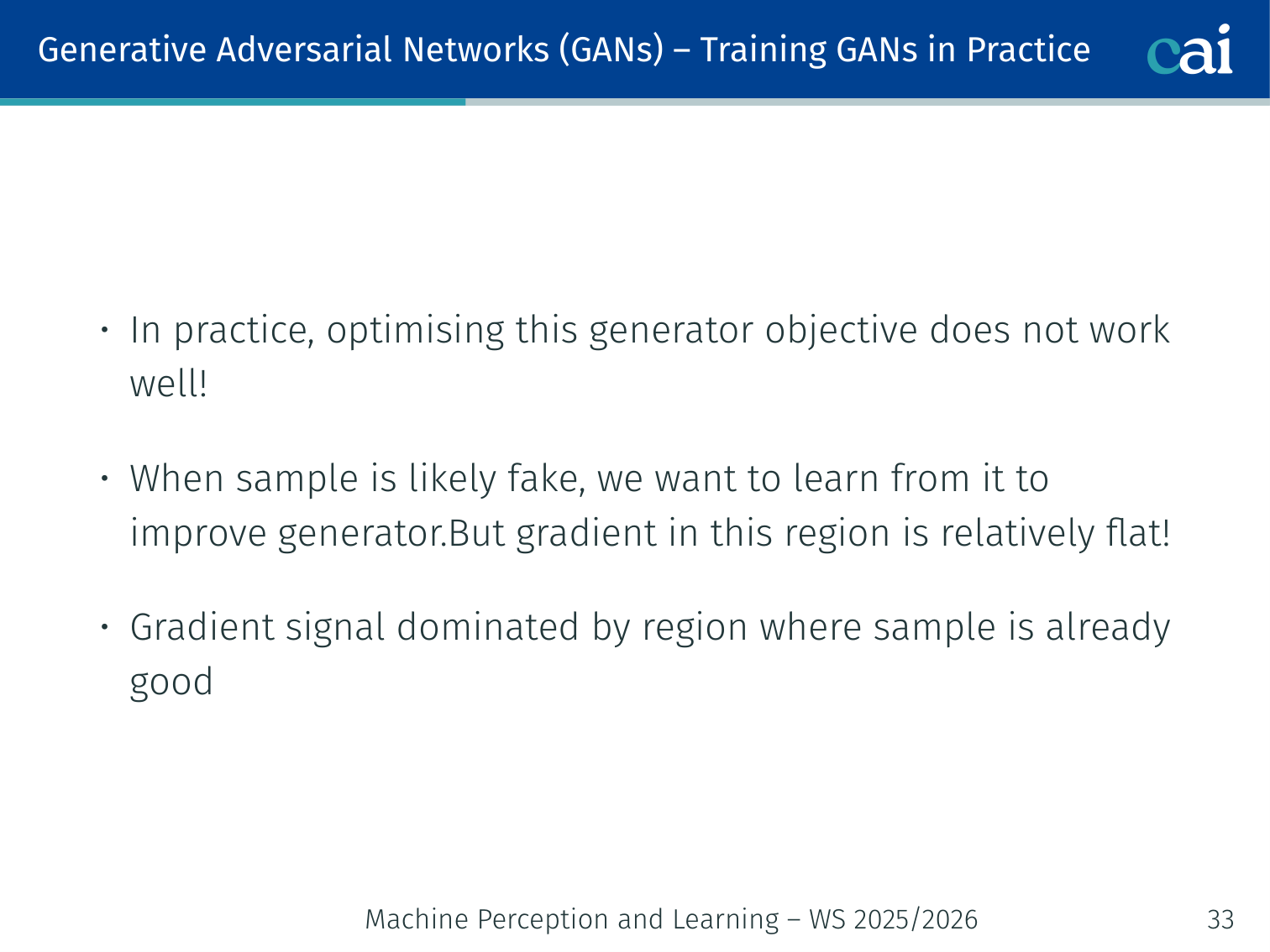
Minimising $\log (1-D(G(z)))$ causes a vanishing gradient early in training:

• When the fake sample is easily detected (likely at the start), $D(G(z))\approx 0$, so $\log (1-D(G(z)))\approx \log 1=0$.
• The gradient in this region is flat — the generator receives almost no learning signal exactly when it needs it most.

The Non-Saturating Fix (Standard in Practice)

Fixing the generator objective so it gets better gradients early on.

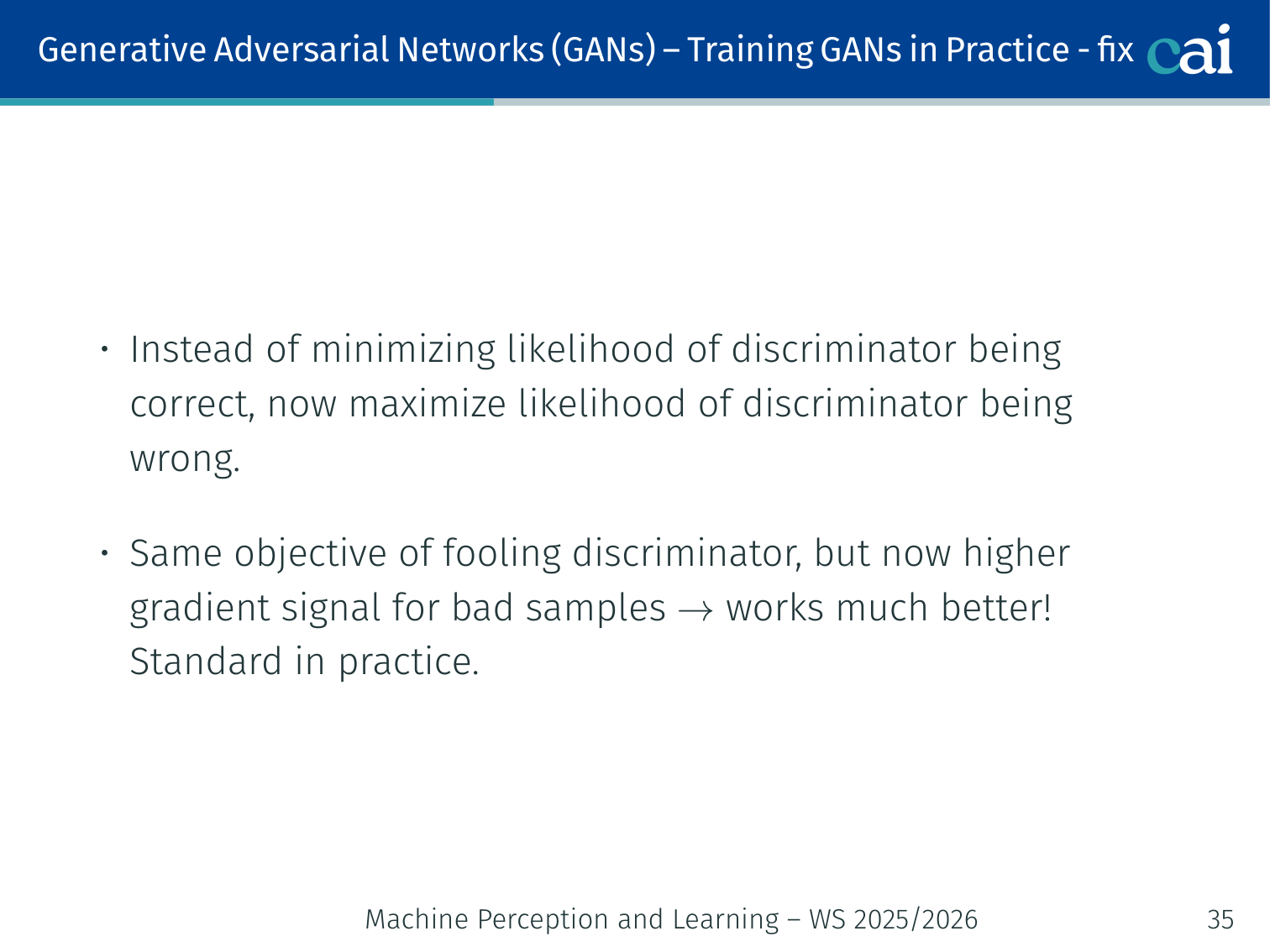
Instead of minimising $\log (1-D(G(z)))$, maximise $\log D(G(z))$:

${\max }_{{\Theta }_g}{\mathbb{E}}_{z\sim p_z}[\log D_{{\Theta }_d}(G_{{\Theta }_g}(z)))]$

Same objective (fool the discriminator), but the gradient is large when the sample is bad — exactly where we need it. This heuristic is standard in virtually all GAN implementations.

Training Loop (PyTorch)

for real_batch in dataloader:
    batch_size = real_batch.size(0)
 
    # ── 1. Train Discriminator (k steps) ──────────────────────────
    for _ in range(k):
        z = torch.randn(batch_size, latent_dim)
        fake = G(z).detach()          # stop gradient flowing to G
 
        real_loss = bce(D(real_batch), torch.ones(batch_size, 1))
        fake_loss = bce(D(fake),       torch.zeros(batch_size, 1))
        d_loss = (real_loss + fake_loss) / 2
 
        optimizer_D.zero_grad()
        d_loss.backward()
        optimizer_D.step()
 
    # ── 2. Train Generator (non-saturating objective) ─────────────
    z = torch.randn(batch_size, latent_dim)
    # We WANT D to output 1 (real) for generated samples
    g_loss = bce(D(G(z)), torch.ones(batch_size, 1))
 
    optimizer_G.zero_grad()
    g_loss.backward()
    optimizer_G.step()

Note: Some implementations use $k=1$ (one D step per G step), others use $k>1$. There is no universally best rule; it depends on the dataset and architecture.

---

Issues

1. Training Instability (Nash Equilibrium)

GAN training is unstable—it's tough to find that perfect Nash equilibrium.

GAN training is a two-player game. Finding a Nash equilibrium is hard: making downhill progress for one player may push the other player uphill.

Additionally, the generator can learn to exploit statistical properties of the discriminator, producing samples that fooled the discriminator but are not actually realistic.

2. Mode Collapse

Mode collapse: when the generator just keeps making the same few things.

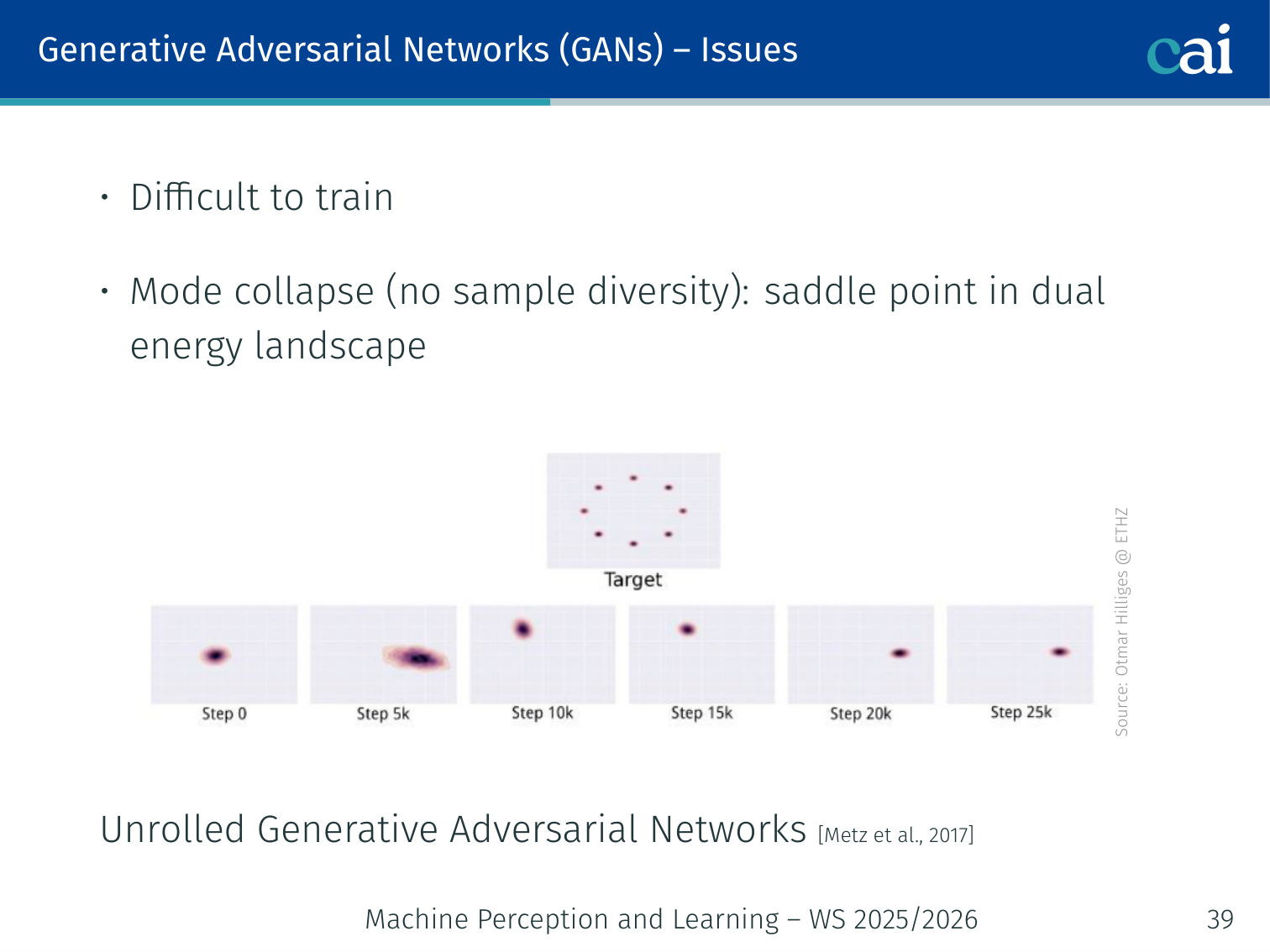
Mode collapse: the generator produces only a small number of outputs (modes) that fool the discriminator, ignoring most of the real data distribution.

Example: A GAN trained on a dataset of handwritten digits (MNIST) might latch onto only “1”s and “3”s because those were easiest to fool the current discriminator, completely ignoring “0”, “2”, “4”–“9”.

Illustrated by a “saddle point in dual energy landscape” — the generator finds a local mode and the discriminator cannot push it away.

Solutions:

• Unrolled GAN (Metz et al., 2017): the generator optimises against a “future” discriminator by unrolling several discriminator update steps.
• Mini-batch discrimination: the discriminator sees entire batches, penalising low sample diversity.
• Wasserstein GAN: different loss that avoids the problem fundamentally (see below).

---

GANs vs VAEs

Comparing VAEs and GANs: training, quality, and how we evaluate density.

Property	VAE	GAN
Training	Relatively easier	Requires many optimisation tricks, prone to mode collapse
Inference	Explicit $q(z\mid x)$	Implicit (no encoder; unless BiGAN)
Image quality	Blurrier (reconstruction loss)	Sharper (discriminator signal)
Density evaluation	Lower bound via ELBO	Not possible — likelihood-free

---

Issues with Jensen-Shannon Divergence

Why Jensen-Shannon Divergence fails when distributions don't overlap.

The JSD-based GAN objective has two serious problems:

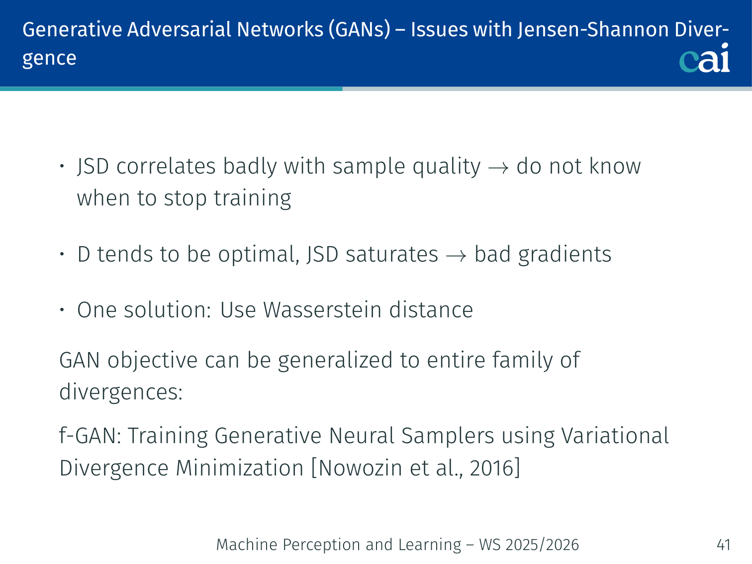
1. JSD correlates poorly with sample quality — you don’t know when to stop training.
2. Gradient vanishing from an optimal discriminator: If $D$ becomes too good, $D_{JSD}$ saturates to $\log 2$ — a constant — and the generator receives zero gradient.

More fundamentally: if $p_{data}$ and $p_G$ have non-overlapping supports (common when the data lies on a low-dimensional manifold of a high-dimensional space), the KL divergence is undefined or infinite, and gradients are not continuous or well-behaved.

Note: The GAN objective can be generalised to an entire family of divergences via f-GAN (Nowozin et al., 2016): Training Generative Neural Samplers using Variational Divergence Minimization.

---

Wasserstein Distance and WGAN

Wasserstein distance: a much more stable objective for training GANs.

Comparing gradients: JSD vs. Wasserstein distance when things are disjoint.

Arjovsky et al., 2017

Earth Mover’s Distance

Visualizing Earth Mover's Distance as the cost of optimal transport between distributions

Intuition for Wasserstein distance using the earth mover's analogy for sand piles

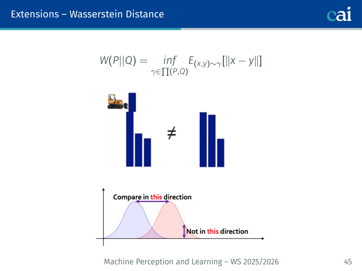
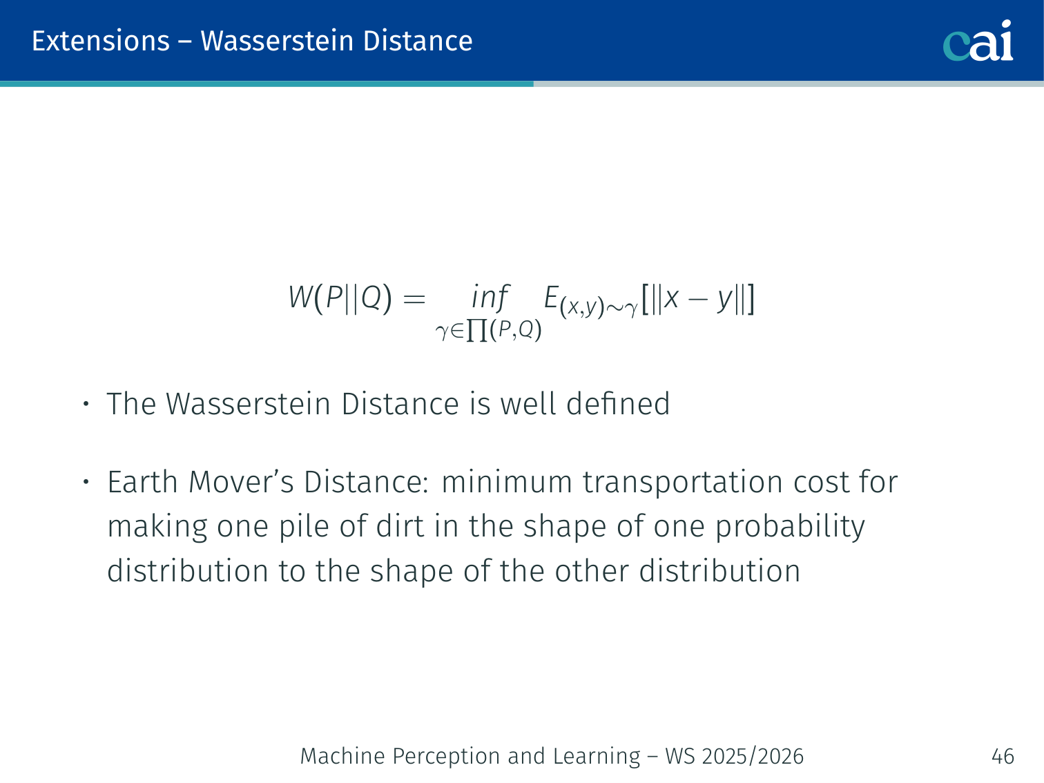
Instead of JSD, use the Wasserstein-1 (Earth Mover’s) Distance:

$W(P\Vert Q)={\inf }_{\gamma \in \Pi (P,Q)}{\mathbb{E}}_{(x,y)\sim \gamma }[\Vert x-y\Vert ]$

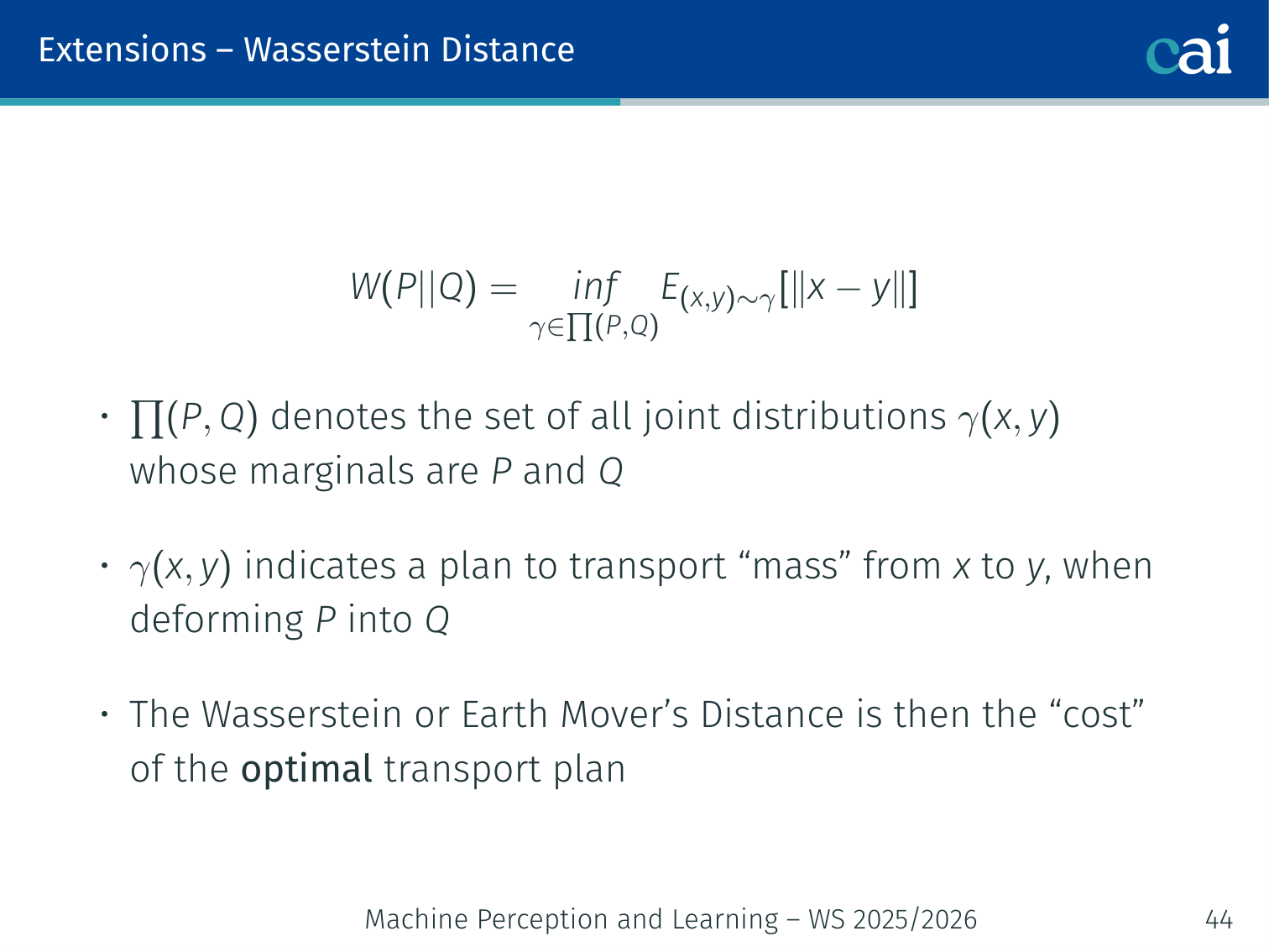
Where $\Pi (P,Q)$ is the set of all joint distributions $\gamma (x,y)$ whose marginals are $P$ and $Q$.

Intuition: the minimum “work” needed to transport a pile of dirt shaped like $P$ to a pile shaped like $Q$. Think of two piles of sand — the Wasserstein distance is the cost of moving sand optimally from one pile’s shape to the other’s.

Why it’s better than JSD:

• Well-defined even when distributions have disjoint support
• Continuous and differentiable everywhere — the generator always gets a useful gradient proportional to how far apart the distributions are

WGAN Objective

By the Kantorovich-Rubinstein duality, the Wasserstein distance can be computed as:

${\min }_G{\max }_{D\in 1\text{-Lip}}{\mathbb{E}}_{x\sim p_{data}}[D(x)]-{\mathbb{E}}_{z\sim p_z}[D(G(z))]$

The discriminator is now called a critic (no sigmoid at the output) and must be 1-Lipschitz (enforced by gradient penalty in WGAN-GP, or weight clipping in the original paper).

# WGAN-GP critic loss
def critic_loss(real, fake, critic, gp_weight=10):
    real_score = critic(real).mean()
    fake_score = critic(fake).mean()
 
    # Gradient penalty (enforce 1-Lipschitz constraint)
    alpha = torch.rand(real.size(0), 1, 1, 1).to(real.device)
    interp = (alpha * real + (1 - alpha) * fake).requires_grad_(True)
    interp_score = critic(interp)
    grads = torch.autograd.grad(interp_score, interp,
                                 grad_outputs=torch.ones_like(interp_score),
                                 create_graph=True)[0]
    gp = ((grads.norm(2, dim=1) - 1) ** 2).mean()
 
    return fake_score - real_score + gp_weight * gp  # minimise this

Benefits of WGAN:

• No mode collapse in practice
• Loss value is meaningful — it correlates with visual sample quality (unlike vanilla GAN loss)
• More stable training

Example: with a vanilla GAN, the loss can oscillate wildly and gives no indication of quality. With WGAN, as training progresses the Wasserstein loss consistently decreases, and you can use it as a reliable stopping criterion.

---

Applications

Conditional GAN (cGAN)

Condition both $G$ and $D$ on an auxiliary label $c$ (class, attribute, etc.) for controlled generation:

${\min }_G{\max }_D{\mathbb{E}}_{x,c}[\log D(x,c)]+{\mathbb{E}}_{z,c}[\log (1-D(G(z,c),c))]$

• Generator: takes $[z;c]$ as input → generates a sample of class $c$
• Discriminator: takes $[x;c]$ as input → judges whether $x$ matches $c$

Example: Train a cGAN on MNIST conditioned on the digit label. At inference, pass $z\sim \mathcal{N}(0,I)$ and $c=7$ to get a generated “7”. You can generate any digit on demand without retraining.

---

Pix2Pix — Image-to-Image Translation

Pix2Pix: using conditional GANs for paired image-to-image translation.

Isola et al., 2017

A conditional GAN where the condition is a full image (not just a label). Requires paired training images $(x,y)$ — e.g., (edge map, photo), (semantic mask, street scene), (day, night).

Objective:

$\mathcal{L}(G,D)={\mathcal{L}}_{cGAN}(G,D)+\lambda {\mathcal{L}}_{L1}(G)$

Where:

${\mathcal{L}}_{cGAN}(G,D)={\mathbb{E}}_{x,y}[\log D(x,y)]+{\mathbb{E}}_{x,z}[1-\log D(x,G(x,z))]$

${\mathcal{L}}_{L1}(G)={\mathbb{E}}_{x,y,z}[\Vert y-G(x,z){\Vert }_1]$

The L1 term encourages low-frequency fidelity; the adversarial term pushes for high-frequency realism.

Input image x ──→ [Generator (U-Net)] ──→ output image ŷ
                                               │
[Discriminator (PatchGAN)] sees (x, y) pairs:
    real pair  (x, y)  → 1
    fake pair  (x, ŷ)  → 0

Applications:

• Sketch → realistic photo
• Semantic segmentation map → street scene photo
• Black & white → colour
• Day photograph → night photograph
• Aerial map → satellite image

Example: Given an architectural blueprint (edge map), Pix2Pix generates a realistic photo of what that building might look like. The discriminator judges whether the photo and the blueprint are a plausible pair, not just whether the photo looks real in isolation.

Limitation: Requires paired images, which are often expensive or impossible to collect (e.g., “photo of an apple” ↔ “photo of an orange”).

---

CycleGAN — Unpaired Image-to-Image Translation

CycleGAN: unpaired translation using cycle-consistency.

Cycle-consistency: from horse to zebra and all the way back to horse.

Zhu et al., 2017

CycleGAN removes the requirement for paired training data. It uses two generators and two discriminators with a cycle-consistency loss.

Setup:

• Domain $X$ (e.g., horses), Domain $Y$ (e.g., zebras)
• Generator $G:X\to Y$, Generator $F:Y\to X$
• Discriminator $D_Y$: real vs. fake in $Y$; Discriminator $D_X$: real vs. fake in $X$

Cycle-consistency: If you translate a horse to a zebra and back, you should get the original horse: $F(G(x))\approx x\text{and}G(F(y))\approx y$

Objective:

$\mathcal{L}(G,F,D_X,D_Y)={\mathcal{L}}_{GAN}(G,D_Y,X,Y)+{\mathcal{L}}_{GAN}(F,D_X,Y,X)+\lambda {\mathcal{L}}_{cyc}(G,F)$

Where the cycle-consistency loss is:

${\mathcal{L}}_{cyc}(G,F)={\mathbb{E}}_{x\sim p_{data}(x)}[\Vert F(G(x))-x{\Vert }_1]+{\mathbb{E}}_{y\sim p_{data}(y)}[\Vert G(F(y))-y{\Vert }_1]$

x (horse) ──→ G ──→ ŷ (fake zebra) ──→ F ──→ x̂ (reconstructed horse)
                                               cycle loss: ||x̂ - x||₁

y (zebra) ──→ F ──→ x̂ (fake horse) ──→ G ──→ ŷ (reconstructed zebra)
                                               cycle loss: ||ŷ - y||₁

Applications:

• Horse ↔ Zebra
• Summer ↔ Winter landscape
• Photo ↔ Monet painting
• Apple ↔ Orange

Example: You have a collection of horse photos and a separate collection of zebra photos — no paired images at all. CycleGAN learns to translate between styles. The cycle-consistency loss prevents the generator from making arbitrary, unrelated changes (e.g., it can’t translate an apple to a zebra and still reconstruct the original apple, so it’s forced to only change the visual style).

---

GauGAN / SPADE — Spatially-Adaptive Normalization

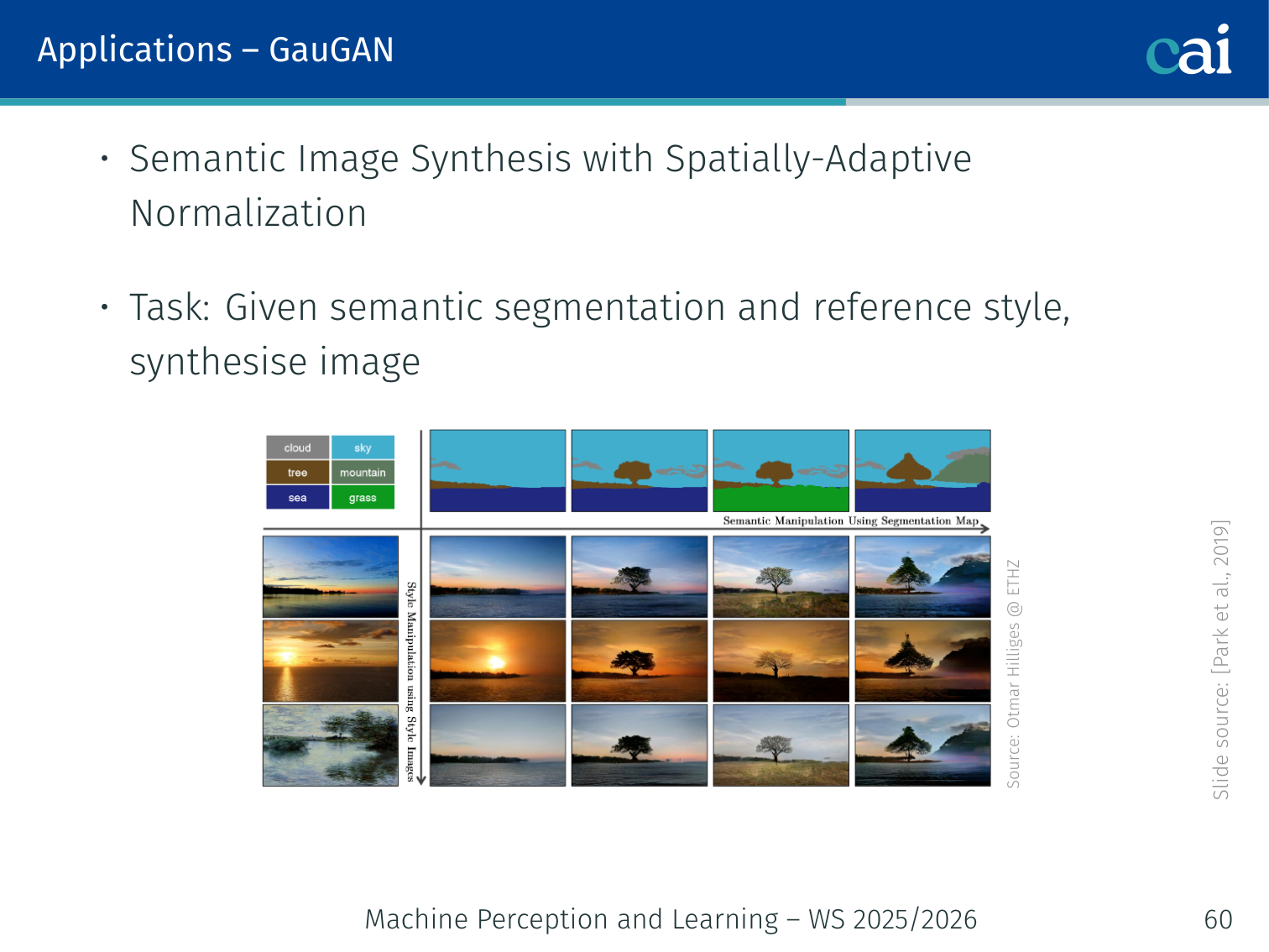
GauGAN: using SPADE to create images from segmentation masks.

Park, Liu, Wang, Zhu (NVIDIA), 2019

Task: Given a semantic segmentation mask and a reference style image, synthesise a photorealistic scene.

Problem with standard conditional normalisation: Unconditional normalisation layers (e.g., BatchNorm) inside the generator “wash away” the semantic label information as activations propagate through the network.

Solution — SPADE (Spatially-Adaptive Denormalization):

Instead of scalar $\gamma$ and $\beta$ vectors, SPADE produces spatially-varying modulation tensors:

1. Project the segmentation mask into an embedding space
2. Apply convolutions to produce $\gamma (x,y)$ and $\beta (x,y)$ — 2D tensors, not just scalars
3. Apply element-wise: normalise the activation, then modulate: $h=\gamma (x,y)\cdot \text{Norm}(h)+\beta (x,y)$

The generator contains a series of SPADE residual blocks with upsampling layers. Each block conditions on the full-resolution semantic map, so spatial information is never lost.

Result: Fine-grained control over what appears where in the generated image.

Example: Draw a rough semantic mask with “sky” at the top, “mountains” in the middle, and “lake” at the bottom. GauGAN renders a photorealistic landscape matching that layout exactly. You can swap the style by providing a different reference image (e.g., a Van Gogh painting) while keeping the same layout.

---

StyleGAN — Style-Based Generator Architecture

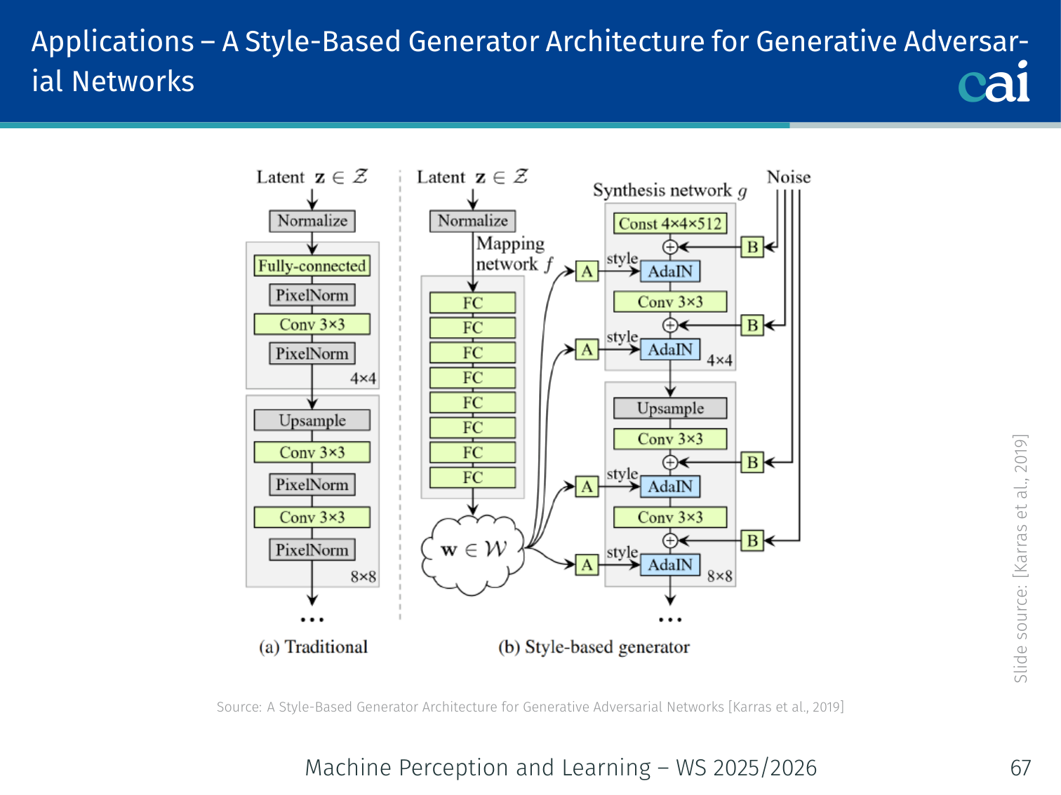
StyleGAN: an overview of the mapping network and AdaIN layers.

Karras, Laine, Aila (NVIDIA), 2019

StyleGAN generates high-resolution photorealistic images (e.g., human faces at 1024×1024) with fine-grained style control.

Key Innovations:

1. Mapping Network

The StyleGAN mapping network: turning noise z into a better latent space w.

$z\sim \mathcal{N}(0,I)$ → 8-layer MLP → $w$ (disentangled latent space)

The $w$-space is more linearly disentangled than $z$-space — individual dimensions correspond more cleanly to interpretable attributes (age, hair, pose, expression, etc.).

2. Adaptive Instance Normalization (AdaIN)

AdaIN: how we inject style directly into the generator.

Style is injected at each resolution by modulating intermediate features:

$\text{AdaIN}(x_i,y)=y_{s,i}\cdot \frac{x_i-\mu (x_i)}{\sigma (x_i)}+y_{b,i}$

Where $y_s,y_b$ are learned affine transforms of $w$. This is how “style” (colour palette, texture, coarse structure) is controlled at each scale.

3. Progressive Growing

Progressive growing: starting small and getting bigger for more stable GANs.

Training starts at low resolution (4×4) and progressively adds layers for higher resolutions (4×4 → 8×8 → 16×16 → … → 1024×1024). This produces stable, high-quality training by starting with easy, coarse structure before refining fine details.

4. Style Mixing

At inference, use $w_1$ for early (coarse) layers and $w_2$ for later (fine) layers. This creates hybrid outputs — e.g., the face shape and pose of person A combined with the hair colour and skin texture of person B.

Style level	Controls
Coarse (4×4–8×8)	Pose, face shape, hair type
Middle (16×16–32×32)	Facial features, eye shape
Fine (64×64–1024×1024)	Colour scheme, micro-texture

Example: thispersondoesnotexist.com generates realistic human faces using StyleGAN. None of the people exist — every image is synthesised from scratch from random $z$ noise. Refresh the page to get a completely different face.

---

Case Study: GANs for Gaze Redirection

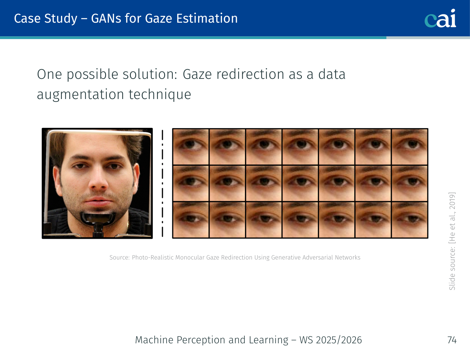
A case study on using GANs for eye gaze redirection.

(He, Spurr, Zhang, Hilliges — ICCV 2019)

Motivation

Appearance-based gaze estimation requires large datasets annotated with ground-truth gaze angles, collected using expensive eye-tracking equipment under diverse conditions (illumination, head pose, gaze angle). Key datasets:

Dataset	Notes
MPIIGaze (Zhang et al., 2015)	In-the-wild appearance-based gaze
GazeCapture (Krafka et al., 2016)	Mobile device eye tracking
ETH-XGaze (Zhang et al., 2020)	Extreme head pose and gaze variation

One solution: Use GANs for gaze redirection as data augmentation — take existing images and synthesise versions with arbitrary target gaze angles.

Task Definition

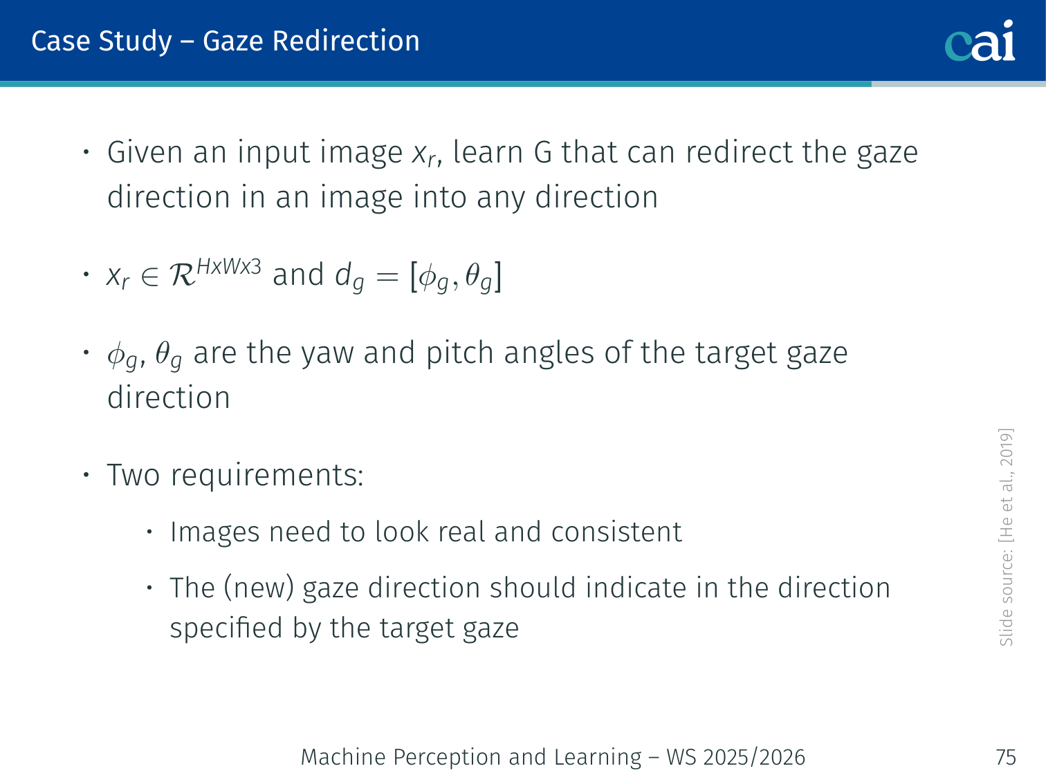
What is gaze redirection? Transforming eyes to look where we want.

Given an input eye image $x_r$ with gaze direction $d_r=[{\varphi }_r,{\theta }_r]$ (yaw, pitch), learn a generator $G$ that redirects the gaze to a target direction $d_g=[{\varphi }_g,{\theta }_g]$:

$G(x_r,d_g)=x_g$

Two requirements:

1. $x_g$ must look photo-realistic and consistent with $x_r$
2. The gaze in $x_g$ must actually point in direction $d_g$

Conditional GAN Framework

The conditional GAN setup for gaze redirection with a dual-purpose discriminator.

The losses we use for gaze redirection: adversarial, gaze, reconstruction, and perceptual.

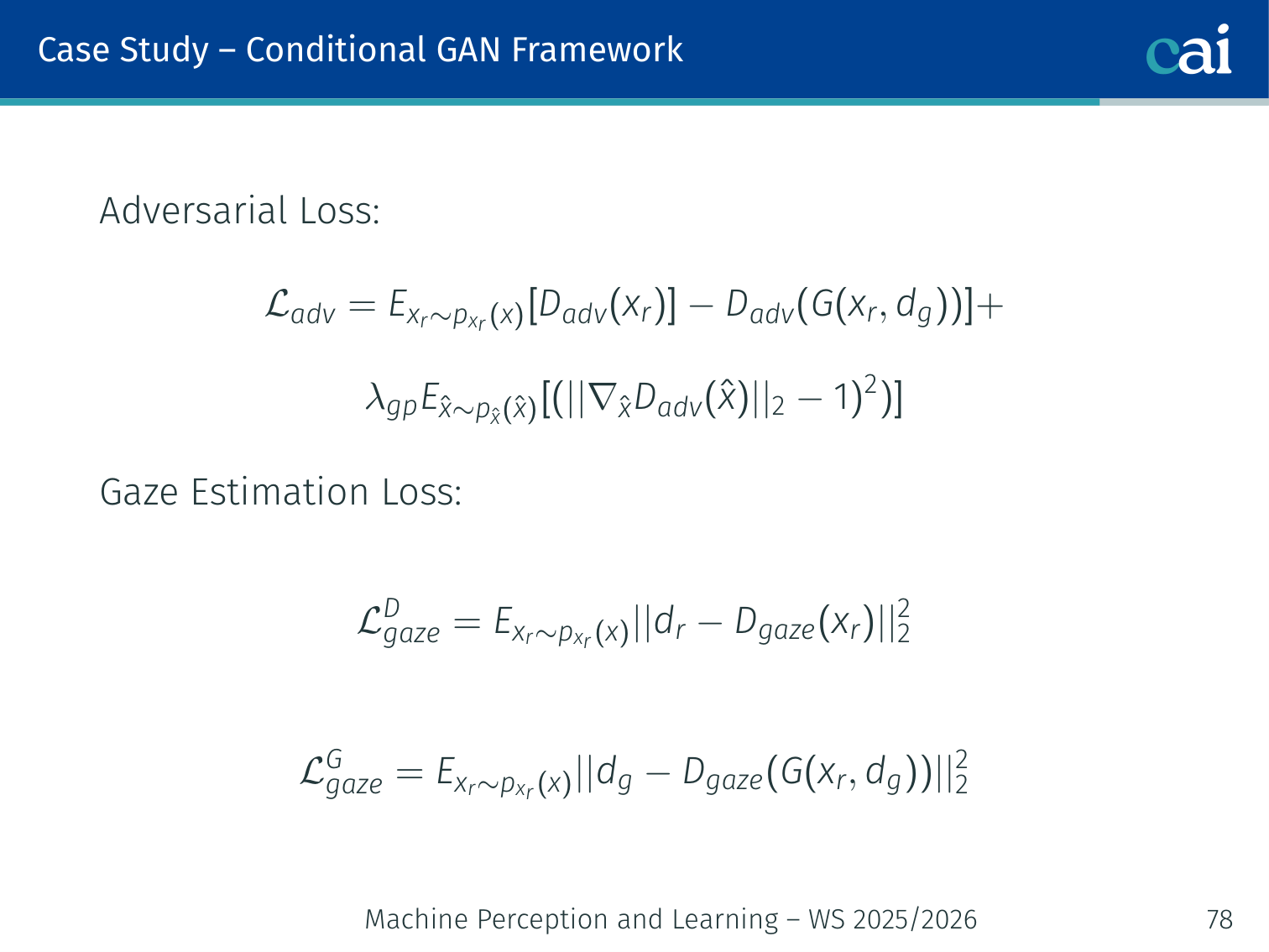
This is the first GAN-based method for monocular gaze redirection. It uses a WGAN-GP framework with a dual-purpose discriminator that simultaneously judges realism and gaze correctness.

1. Adversarial Loss (Wasserstein with gradient penalty):

${\mathcal{L}}_{adv}={\mathbb{E}}_{x_r\sim p_{x_r}}[D_{adv}(x_r)]-D_{adv}(G(x_r,d_g))+{\lambda }_{gp}{\mathbb{E}}_{\hat{x}\sim p_{\hat{x}}}[(\Vert {\nabla }_{\hat{x}}{D}_{adv}(\hat{x}){\Vert }_2-1{)}^2]$

2. Gaze Estimation Loss (discriminator also acts as a gaze estimator):

${\mathcal{L}}_{gaze}^D={\mathbb{E}}_{x_r\sim p_{x_r}}\Vert d_r-D_{gaze}(x_r){\Vert }_2^2$

${\mathcal{L}}_{gaze}^G={\mathbb{E}}_{x_r\sim p_{x_r}}\Vert d_g-D_{gaze}(G(x_r,d_g)){\Vert }_2^2$

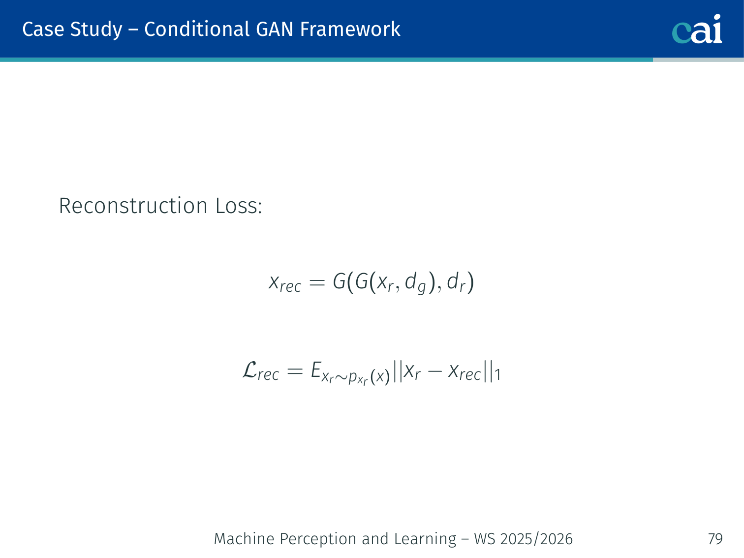
3. Reconstruction Loss (cycle-consistency — redirect then redirect back):

$x_{rec}=G(G(x_r,d_g),d_r){\mathcal{L}}_{rec}={\mathbb{E}}_{x_r}[\Vert x_r-x_{rec}{\Vert }_1]$

4. Perceptual Loss (using VGG-16 features, inspired by Johnson et al., 2016):

${\mathcal{L}}_c={\mathbb{E}}_{x_r}\left[\frac{1}{H_j{W}_j{C}_j}\Vert {\psi }_j(G(x_r,d_g))-{\psi }_j(x_t){\Vert }^2\right]$

${\mathcal{L}}_s={\mathbb{E}}_{x_r}\left[{\sum }_{j=1}^J\Vert f_j(G(x_r,d_g))-f_j(x_t){\Vert }^2\right]$

Where ${\psi }_j$ is the $j$-th activation of a pretrained VGG-16, and $f_j$ is the Gram matrix (captures style/texture).

Overall Objectives

${\mathcal{L}}_G=-{\mathcal{L}}_{adv}+{\lambda }_p{\mathcal{L}}_p+{\lambda }_{gaze}{\mathcal{L}}_{gaze}^G+{\lambda }_{rec}{\mathcal{L}}_{rec}$

${\mathcal{L}}_D={\mathcal{L}}_{adv}+{\lambda }_{gaze}{\mathcal{L}}_{gaze}^D$

Evaluation Metric: LPIPS

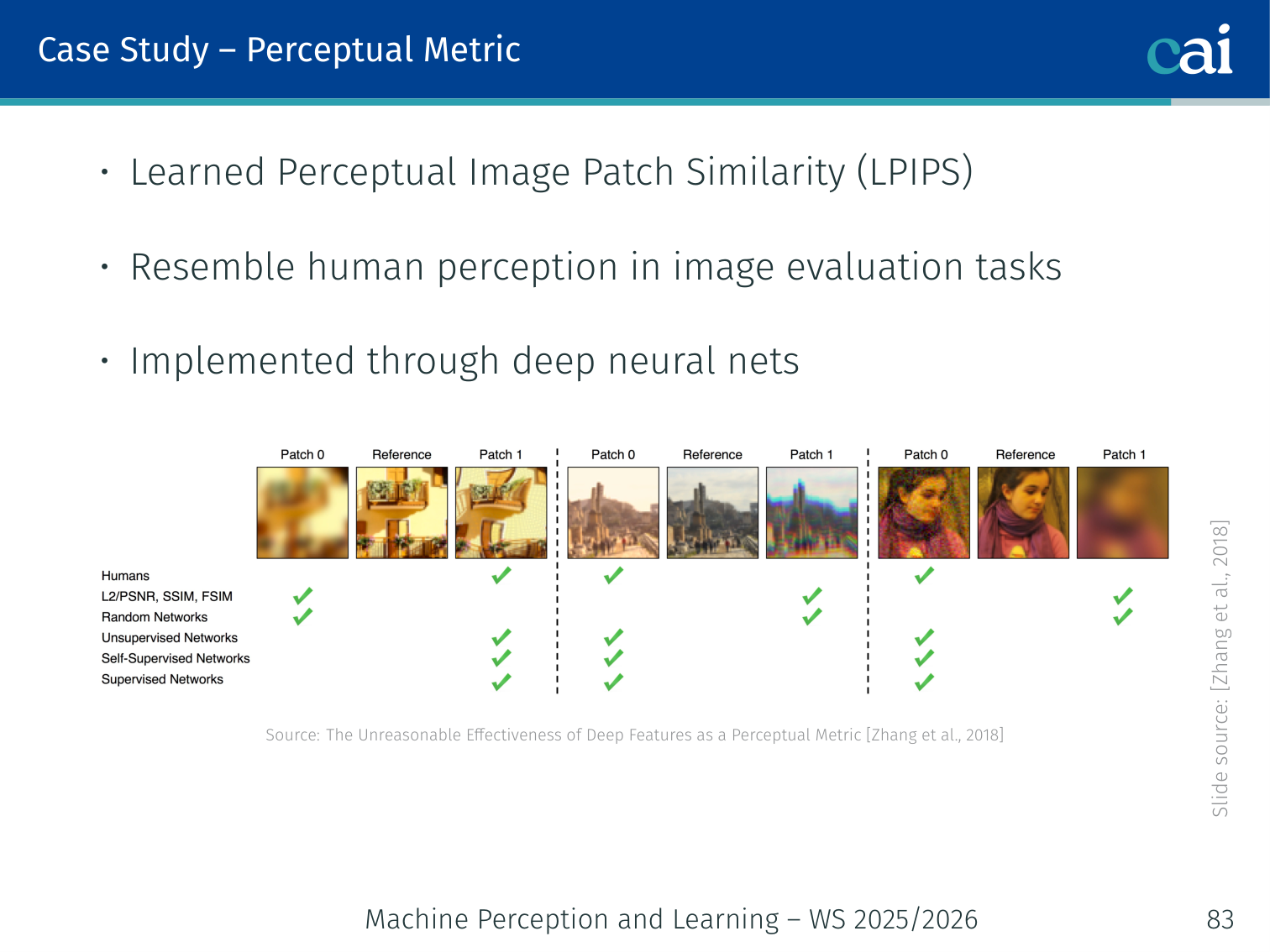
LPIPS: a learned metric for comparing how similar image patches look.

Perceptual quality is evaluated using LPIPS (Learned Perceptual Image Patch Similarity, Zhang et al., 2018):

• Uses deep neural network features to compare images
• Designed to match human perceptual judgements
• Better than pixel-wise metrics (PSNR, SSIM) for evaluating generated image quality

Key Contributions

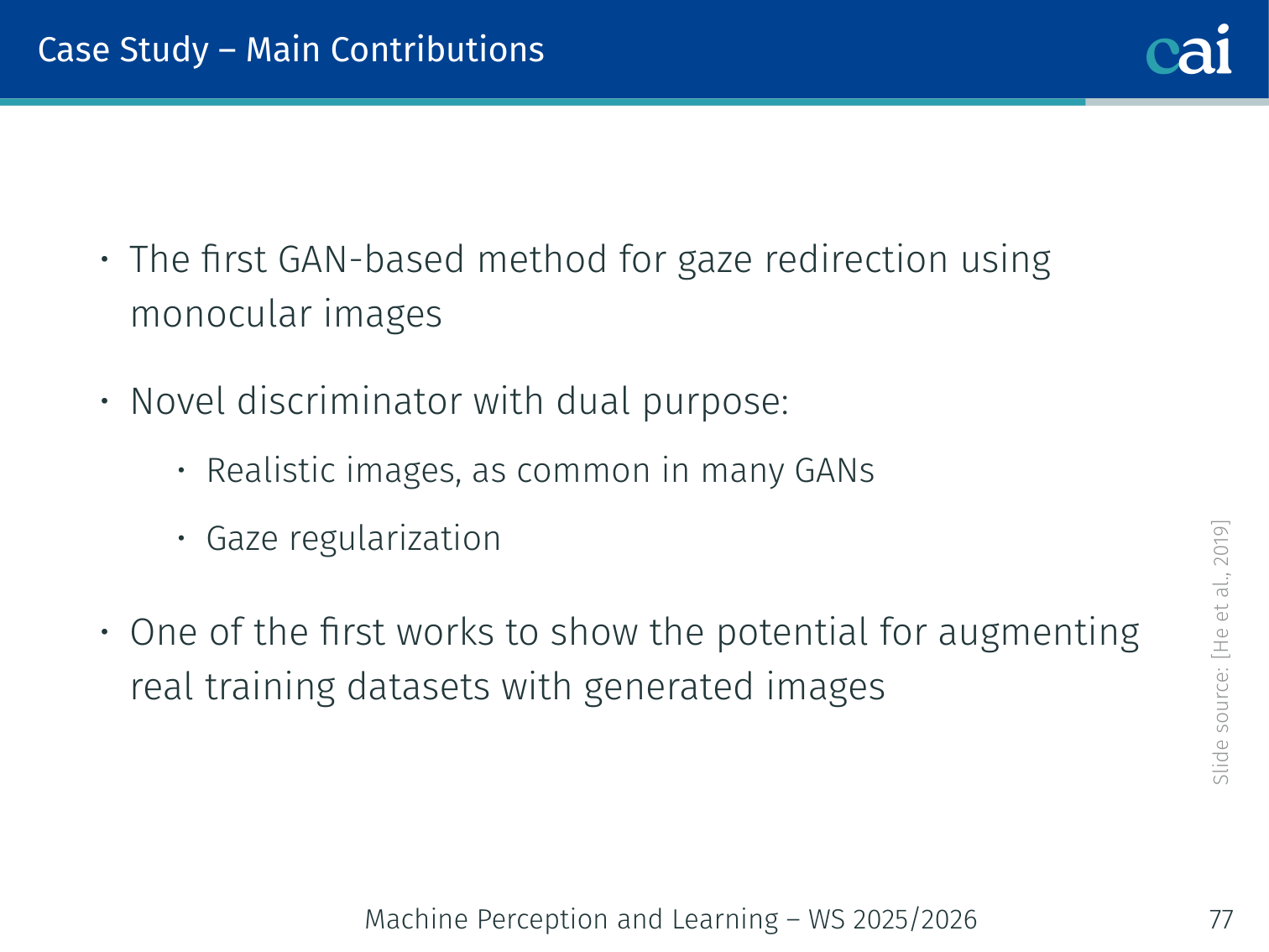
A wrap-up of the key takeaways from the gaze redirection case study.

1. First GAN-based method for gaze redirection from monocular images
2. Novel dual-purpose discriminator — judges both realism and gaze direction
3. One of the first works to demonstrate synthetic image augmentation improving real gaze estimation model performance

---

Evaluation Metrics for GANs

Metric	Measures	Direction
FID (Fréchet Inception Distance)	Distributional similarity to real data	Lower is better
IS (Inception Score)	Quality + diversity jointly	Higher is better
LPIPS	Perceptual similarity to a reference	Lower is better
Precision & Recall	Quality vs. diversity separately	Both higher

FID — The Standard Metric

Extract InceptionV3 features from real and generated images. Fit Gaussians to each feature set. Compute:

$\text{FID}=\Vert {\mu }_r-{\mu }_g{\Vert }^2+\text{Tr}\left({\Sigma }_r+{\Sigma }_g-2({\Sigma }_r{\Sigma }_g{)}^{1/2}\right)$

Lower FID means the generated distribution is closer to the real one. FID captures both quality (fidelity) and diversity, making it the de facto standard.

Example: A mode-collapsed GAN that generates only one type of face might have high per-image quality but terrible FID, because its distribution barely overlaps with the full real data distribution. IS might still give it a decent score. FID reliably catches both issues.

---

Summary: GAN Variants

GAN Variant	Key Innovation	Paper
Vanilla GAN	Minimax game, JS divergence	Goodfellow et al., 2014
DCGAN	Convolutional architecture, BatchNorm	Radford et al., 2015
WGAN / WGAN-GP	Wasserstein distance, stable training	Arjovsky et al., 2017
cGAN	Condition on labels for controlled generation	Mirza & Osindero, 2014
Pix2Pix	Condition on paired images	Isola et al., 2017
CycleGAN	Unpaired translation via cycle-consistency	Zhu et al., 2017
GauGAN / SPADE	Spatially-adaptive normalization	Park et al., 2019
StyleGAN	Disentangled $w$-space, AdaIN	Karras et al., 2019

Final Comparison: VAEs vs GANs

	VAE	GAN
Training	Easier (single optimisation)	Hard (adversarial, mode collapse risk)
Inference	Explicit $q(z\mid x)$	Implicit
Image quality	Blurry	Sharp
Density access	Lower bound	None (likelihood-free)

GANs have largely been superseded by diffusion models for highest-quality generation, but adversarial training and discriminators remain influential — appearing in perceptual loss networks, data augmentation pipelines, and as discriminators in hybrid models.

PyTorch Implementation: DCGAN

Deep Convolutional GANs (DCGAN) replaced the standard MLPs of the original GAN with convolutional layers, greatly improving stability and image quality.

import torch
import torch.nn as nn
 
# 1. The GENERATOR: Maps noise 'z' to an Image
class Generator(nn.Module):
    def __init__(self, nz=100, ngf=64, nc=1):
        super().__init__()
        self.main = nn.Sequential(
            # Input is noise z, shape (Batch, 100, 1, 1)
            # ConvTranspose2d performs UPSAMPLING
            nn.ConvTranspose2d(nz, ngf * 4, 4, 1, 0, bias=False),
            nn.BatchNorm2d(ngf * 4),
            nn.ReLU(True),
 
            # Upsample to 8x8
            nn.ConvTranspose2d(ngf * 4, ngf * 2, 4, 2, 1, bias=False),
            nn.BatchNorm2d(ngf * 2),
            nn.ReLU(True),
 
            # Upsample to 16x16
            nn.ConvTranspose2d(ngf * 2, ngf, 4, 2, 1, bias=False),
            nn.BatchNorm2d(ngf),
            nn.ReLU(True),
 
            # Final layer maps to 32x32 image (nc=3 for RGB, 1 for Grayscale)
            nn.ConvTranspose2d(ngf, nc, 4, 2, 1, bias=False),
            # Tanh scales output pixels to [-1, 1]
            nn.Tanh()
        )
 
    def forward(self, x):
        return self.main(x)
 
# 2. The DISCRIMINATOR: Maps an Image to a Probability [0, 1]
class Discriminator(nn.Module):
    def __init__(self, nc=1, ndf=64):
        super().__init__()
        self.main = nn.Sequential(
            # Standard Conv2d performs DOWNSAMPLING
            # Input: (Batch, nc, 32, 32)
            nn.Conv2d(nc, ndf, 4, 2, 1, bias=False),
            # LeakyReLU is standard for GAN discriminators
            nn.LeakyReLU(0.2, inplace=True),
 
            nn.Conv2d(ndf, ndf * 2, 4, 2, 1, bias=False),
            nn.BatchNorm2d(ndf * 2),
            nn.LeakyReLU(0.2, inplace=True),
 
            # Final convolution reduces to a 1x1 scalar
            nn.Conv2d(ndf * 2, 1, 7, 1, 0, bias=False),
            # Sigmoid outputs probability of image being REAL
            nn.Sigmoid()
        )
 
    def forward(self, x):
        # Flatten the output to a single dimension (Batch_size,)
        return self.main(x).view(-1)

Key GAN Concepts:

• Upsampling vs. Downsampling: The Generator uses ConvTranspose2d to turn a small noise vector into a large image. The Discriminator uses standard Conv2d to condense an image into a single “real or fake” score.
• Binary Cross-Entropy (BCE): GANs are typically trained with BCE. The Discriminator wants to output 1 for real images and 0 for fake ones. The Generator wants to trick it into outputting 1 for fakes.
• Batch Normalization: Essential for preventing the GAN from collapsing into a single output mode early in training.

---

Further Reading

• GAN Zoo (hundreds of GAN variants): https://github.com/hindupuravinash/the-gan-zoo
• Tips and tricks for training GANs: https://github.com/soumith/ganhacks

---

References

• Goodfellow, Pouget-Abadie, Mirza, Xu, Warde-Farley, Ozair, Courville, Bengio (2014). Generative Adversarial Nets. NeurIPS.
• Arjovsky, Chintala, Bottou (2017). Wasserstein GAN. arXiv:1701.07875.
• Isola, Zhu, Zhou, Efros (2017). Image-to-Image Translation with Conditional Adversarial Networks. CVPR.
• Zhu, Park, Isola, Efros (2017). Unpaired Image-to-Image Translation using Cycle-Consistent Adversarial Networks. ICCV.
• Park, Liu, Wang, Zhu (2019). Semantic Image Synthesis with Spatially-Adaptive Normalization. CVPR.
• Karras, Laine, Aila (2019). A Style-Based Generator Architecture for Generative Adversarial Networks. CVPR.
• He, Spurr, Zhang, Hilliges (2019). Photo-Realistic Monocular Gaze Redirection Using Generative Adversarial Networks. ICCV.
• Metz, Poole, Pfau, Sohl-Dickstein (2017). Unrolled Generative Adversarial Networks. arXiv:1611.02163.
• Nowozin, Cseke, Tomioka (2016). f-GAN: Training Generative Neural Samplers using Variational Divergence Minimization. NIPS.
• Zhang, Isola, Efros, Shechtman, Wang (2018). The Unreasonable Effectiveness of Deep Features as a Perceptual Metric. CVPR.
• Zhang, Sugano, Fritz, Bulling (2015). Appearance-Based Gaze Estimation in the Wild. CVPR.
• Krafka, Khosla, Kellnhofer et al. (2016). Eye Tracking for Everyone. CVPR.
• Zhang, Park, Beeler, Bradley, Tang, Hilliges (2020). ETH-XGaze: A Large Scale Dataset for Gaze Estimation under Extreme Head Pose and Gaze Variation. ECCV.

Applied Exam Focus

• Min-Max Game: The Generator tries to fool the Discriminator, while the Discriminator tries to distinguish real from fake. This is a Nash Equilibrium problem.
• Mode Collapse: Occurs when the Generator discovers a single “safe” output that fools the Discriminator and stops producing diverse samples.
• WGAN: Uses the Earth Mover (Wasserstein) Distance to provide smoother gradients even when the real and fake distributions don’t overlap.

---

Previous: L09 — VAE | Back to MPL Index | Next: (y-11) RL | (y) Return to Notes | (y) Return to Home