L11 — Reinforcement Learning

Previous: L10 — GANs | Back to MPL Index | Next: (y-12) Diffusion

---

University of Stuttgart — Machine Perception and Learning for Collaborative Intelligent Systems, Prof. Dr. Andreas Bulling, WS 2025/2026

Goal of this lecture: Go from first principles all the way to PPO — one of the most widely used RL algorithms today.

---

Mental Model First

• RL is about delayed credit assignment: an action now may only reveal its value much later.
• Value functions estimate how promising a state or action is in the long run; policies decide what to do next.
• Many RL algorithms differ mainly in how they trade off exploration, stability, variance, and sample efficiency.
• If one question guides this lecture, let it be: how do we learn from sparse, delayed rewards when the correct action is not labeled for us?

Introduction

Three Paradigms of Learning

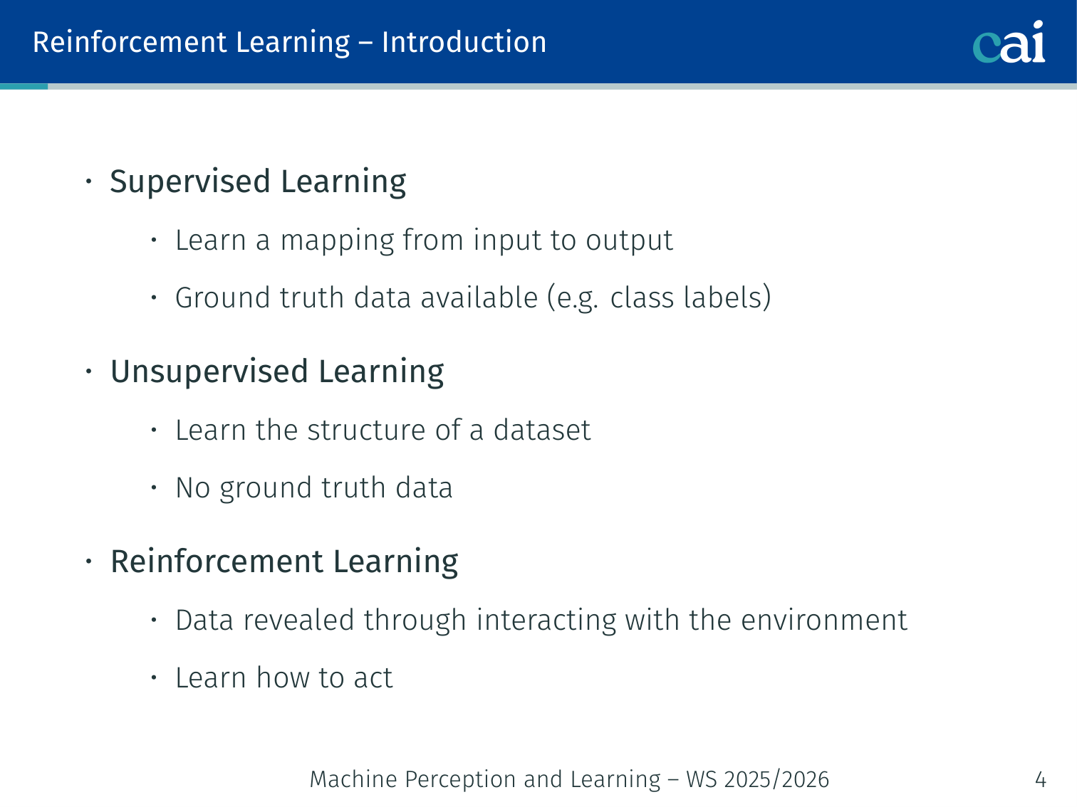
The three paradigms: supervised, unsupervised, and reinforcement learning.

Paradigm	How it learns	Data
Supervised Learning	Learn a mapping from input to output	Ground truth labels available
Unsupervised Learning	Learn the structure of a dataset	No ground truth
Reinforcement Learning	Data revealed through interacting with an environment	Learn how to act

Informally:

• SL: “This is a cat.”
• UL: “These two images look similar.”
• RL: “This cat likes to be scratched behind the ears.” (discovered through interaction)

The RL Problem

Reinforcement learning: learning through trial and error.

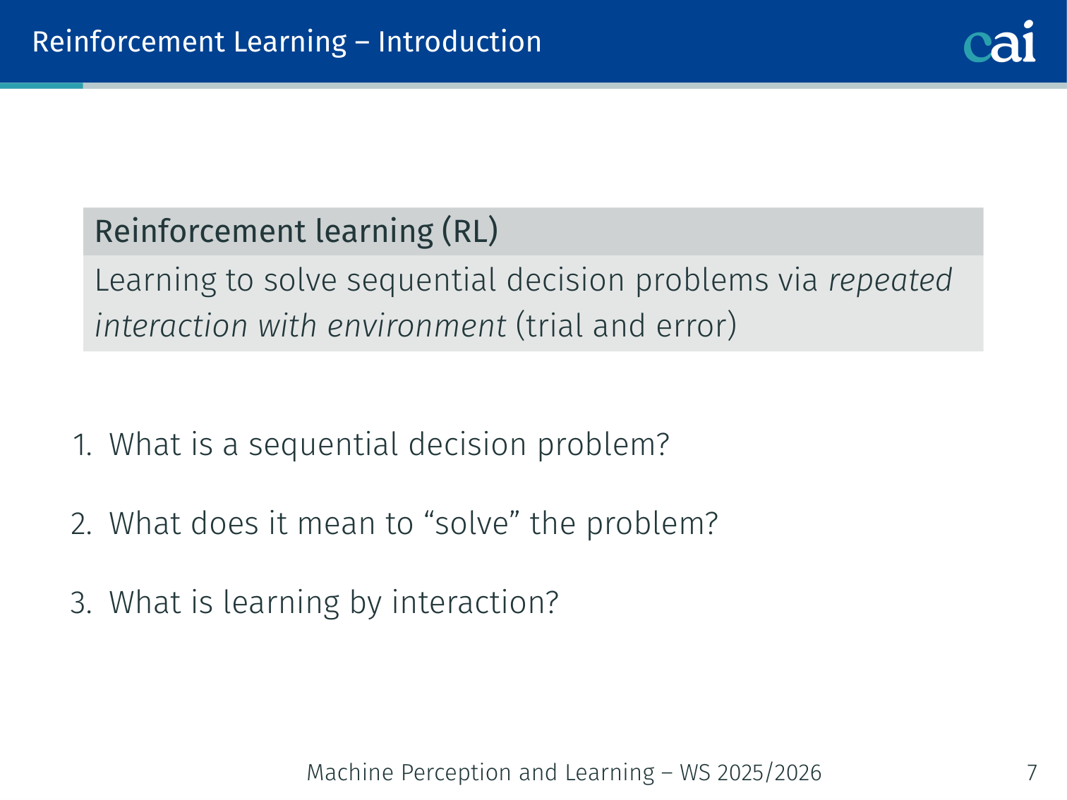
Reinforcement learning is learning to solve sequential decision problems via repeated interaction with an environment (trial and error).

Three questions to answer:

1. What is a sequential decision problem? → MDP
2. What does it mean to “solve” it? → Maximise total reward
3. What is learning by interaction? → TD / Policy Gradient

The Agent–Environment Loop

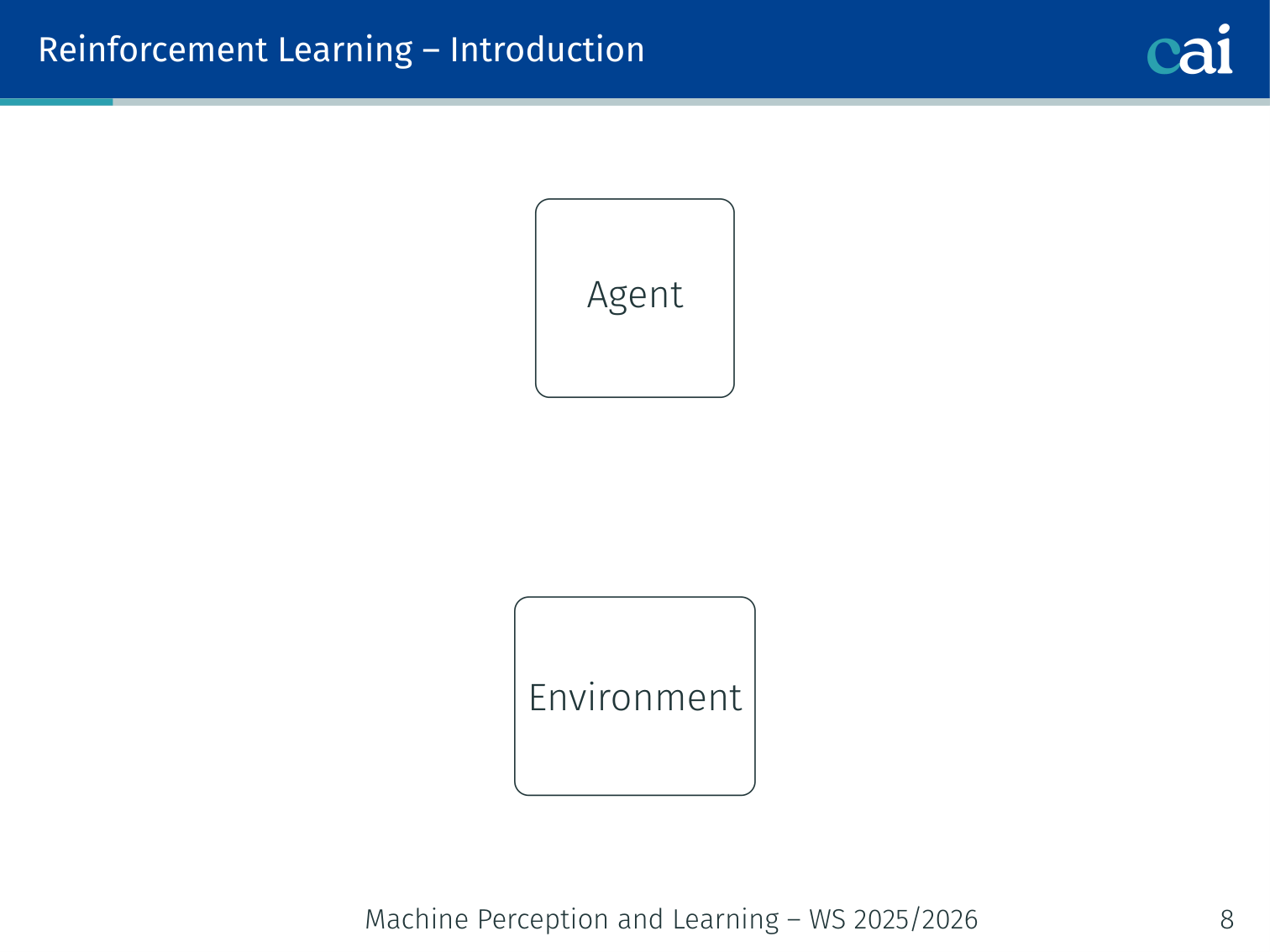
The RL loop: agent and environment in a constant exchange.

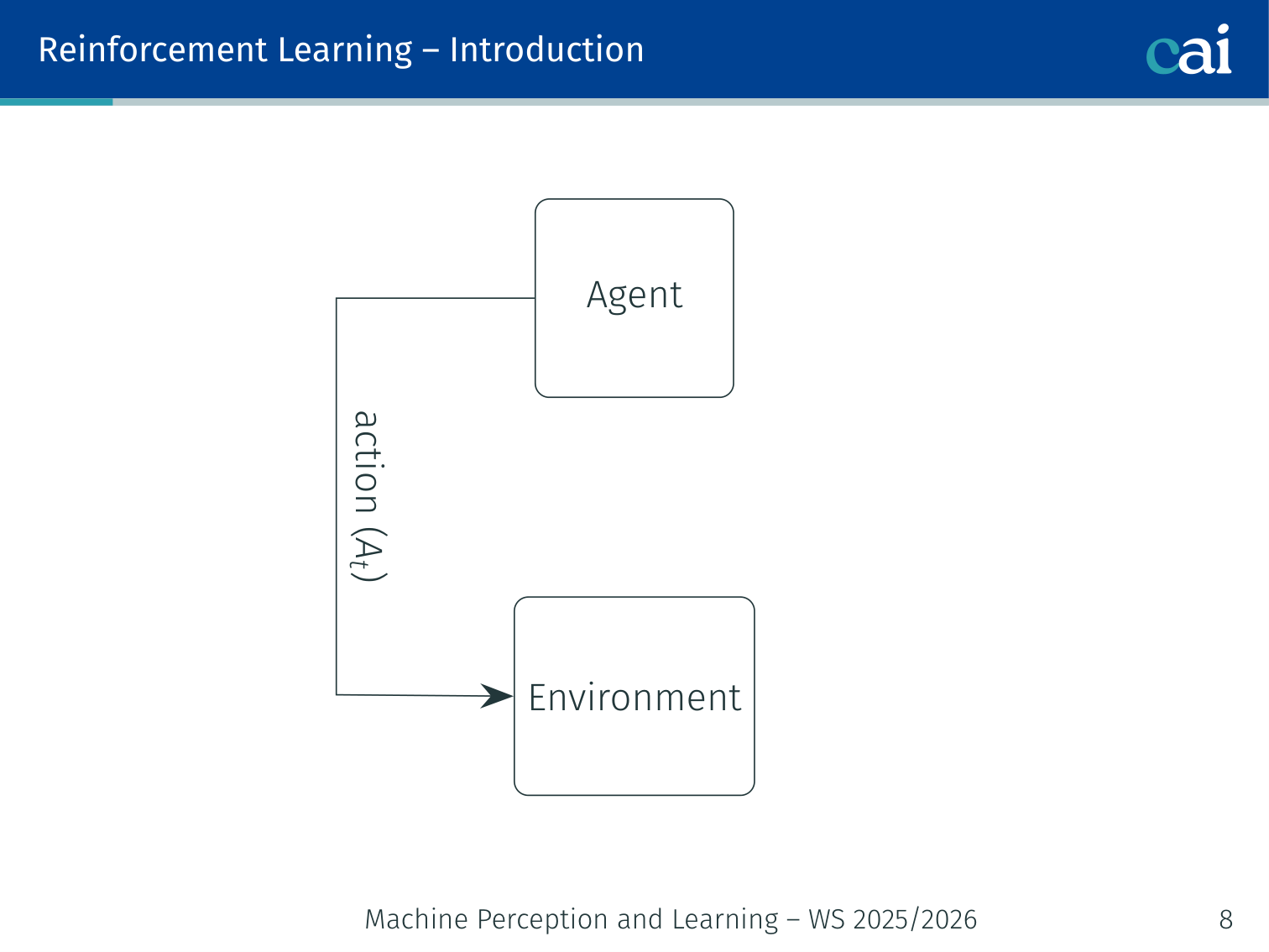
A simple diagram of how state, action, and reward flow in RL.

     +-----------------------------------+
     |            Agent                  |
     |         Policy π(a|s)             |
     +----------------+------------------+
                      | action (At)
                      v
     +-----------------------------------+
     |          Environment              |
     |   state (St)    reward (Rt)       |
     +-----------------------------------+

At each timestep $t$:

1. Agent observes state $s_t$
2. Agent selects action $a_t\sim \pi (\cdot |s_t)$
3. Environment transitions to $s_{t+1}$ and emits reward $r_{t+1}$
4. Agent uses $(s_t,a_t,r_{t+1},s_{t+1})$ to update its policy

---

💡 Intuition: Reinforcement Learning as “Puppy Training”

Imagine you are teaching a puppy to sit.

1. Observation: The puppy is standing (the State).
2. Action: The puppy sits down (the Action).
3. Reward: You give it a treat (the Reward).
4. Learning: Next time the puppy is in that state, it’s much more likely to sit because it remembers the treat.

The important thing is that you never tell the puppy how to move its muscles. You just reward the outcome. This is why RL is so powerful for things like walking robots — we don’t have to program the exact movement; the robot “discovers” it through trial and error.

---

🧠 Deep Dive: Why the “Advantage” Function?

In basic Policy Gradient (REINFORCE), we use the total reward $G$ to tell the model: “This whole episode was good.”

The Problem: Some actions in a good episode might actually have been bad. (E.g., you won a game of chess, but you made one terrible move in the middle).

The Solution: The Advantage Function $A(s,a)=Q(s,a)-V(s)$.

• It doesn’t just ask: “Was this a good action?”
• It asks: “Was this action better than average for this state?”

If the average reward for being in state $s$ is 10, and your action leads to a reward of 12, the Advantage is $+2$. If it leads to 8, the Advantage is $-2$ (even though 8 is still positive!). This tells the model to only boost the actions that outperform our current expectations.

---

Markov Decision Process (MDP)

Formal Definition

A formal look at MDPs: the foundation of RL math.

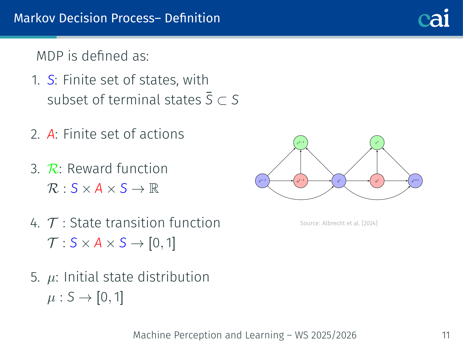
An MDP is the tuple $(S,A,R,T,\mu )$:

Symbol	Meaning
$S$	Finite set of states (with terminal subset $\bar{S}\subseteq S$)
$A$	Finite set of actions
$R:S\times A\times S\to \mathbb{R}$	Reward function
$T:S\times A\times S\to [0,1]$	State-transition function $p(s^{\prime }\mid s,a)$
$\mu :S\to [0,1]$	Initial state distribution

The Markov property: the future depends only on the current state, not history: $p(s_{t+1}|s_t,a_t,s_{t-1},a_{t-1},\dots )=p(s_{t+1}|s_t,a_t)$

Expected Discounted Return

Calculating the expected return, with a bit of a discount for the future.

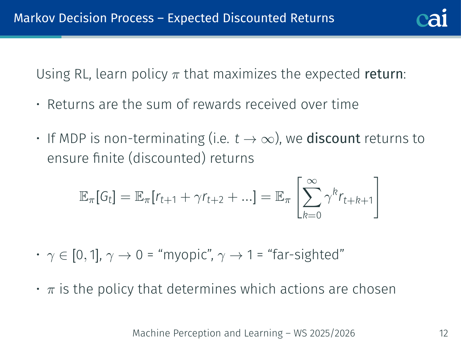
The goal is to learn a policy $\pi$ that maximises the expected discounted return:

${\mathbb{E}}_{\pi }[G_t]={\mathbb{E}}_{\pi }\left[{\sum }_{k=0}^{\infty }{\gamma }^k{r}_{t+k+1}\right]$

• $\gamma \to 0$: myopic — only cares about immediate reward
• $\gamma \to 1$: far-sighted — weights all future rewards nearly equally

Example: Rewards of $1,1,1,\dots$ forever. With $\gamma =0.9$: $G=\frac{1}{1-0.9}=10$. Without discounting $(\gamma =1)$ the sum diverges.

Value Functions

Value functions: what's a state or action actually worth?

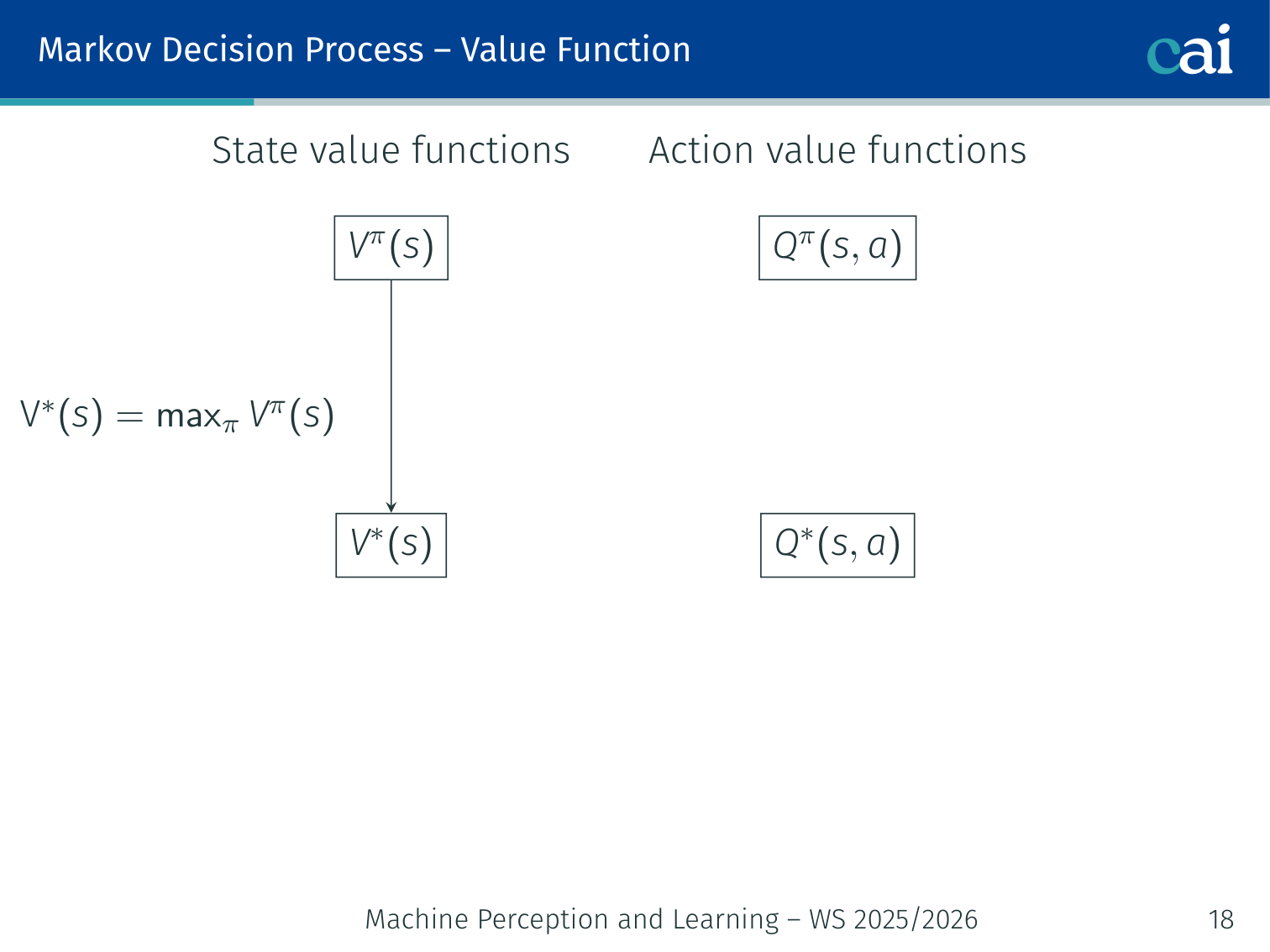
State-value function: $V^{\pi }(s)={\mathbb{E}}_{\pi }[G_t\mid S_t=s]$

Optimal: $V^{\ast }(s)={\max }_{\pi }{V}^{\pi }(s)$

Action-value function: $Q^{\pi }(s,a)={\mathbb{E}}_{\pi }[G_t\mid S_t=s,A_t=a]$

Optimal: $Q^{\ast }(s,a)={\max }_{\pi }{Q}^{\pi }(s,a)$

Key relationships: $V^{\pi }(s)={\sum }_a\pi (a|s)Q^{\pi }(s,a)V^{\ast }(s)={\max }_a{Q}^{\ast }(s,a)$

Optimal policy derived from $Q^{\ast }$: ${\pi }^{\ast }(a|s)=\{\begin{array}{ll}1& \text{if }a=\arg {\max }_{a^{\prime }}{Q}^{\ast }(s,a^{\prime })\\ 0& \text{otherwise}\end{array}$

Or via one-step look-ahead using $V^{\ast }$: ${\pi }^{\ast }(a|s)=\{\begin{array}{ll}1& a=\arg {\max }_{a^{\prime }}\left[{\sum }_{s^{\prime }}p(s^{\prime }|s,a^{\prime })(r(s,a^{\prime },s^{\prime })+\gamma V^{\ast }(s^{\prime }))\right]\\ 0& \text{otherwise}\end{array}$

Bellman Equation

The return decomposes recursively: $G_t=r_{t+1}+\gamma G_{t+1}$. Taking expectations:

$\boxed{V^{\pi }(s)=\sum _a\pi (a|s)\sum _{s^{\prime }}p(s^{\prime }|s,a)\left[r(s,a,s^{\prime })+\gamma V^{\pi }(s^{\prime })\right]}$

$Q^{\pi }(s,a)={\sum }_{s^{\prime }}p(s^{\prime }|s,a)\left(r(s,a,s^{\prime })+\gamma {\sum }_{a^{\prime }}\pi (a^{\prime }|s^{\prime })Q^{\pi }(s^{\prime },a^{\prime })\right)$

We can solve for $V^{\pi }$ iteratively: $V_{[k+1]}^{\pi }(s)={\sum }_a\pi (a|s){\sum }_{s^{\prime }}p(s^{\prime }|s,a)\left[r(s,a,s^{\prime })+\gamma V_{[k]}^{\pi }(s^{\prime })\right]$

💡 Intuition: Bellman Means “Immediate Reward + Future Promise”

The Bellman equation says the value of a state is not mysterious. It is just:

1. what you expect to get right now
2. plus what you expect the next state to be worth

That is why RL can use bootstrapping. Instead of waiting until the whole future has happened, it can reuse its current guess of the future as part of the target.

Sutton and Barto describe this as a recursive relationship between a state and its successor states. That recursive structure is the backbone of dynamic programming, TD learning, Q-learning, and actor-critic methods.

---

Dynamic Programming

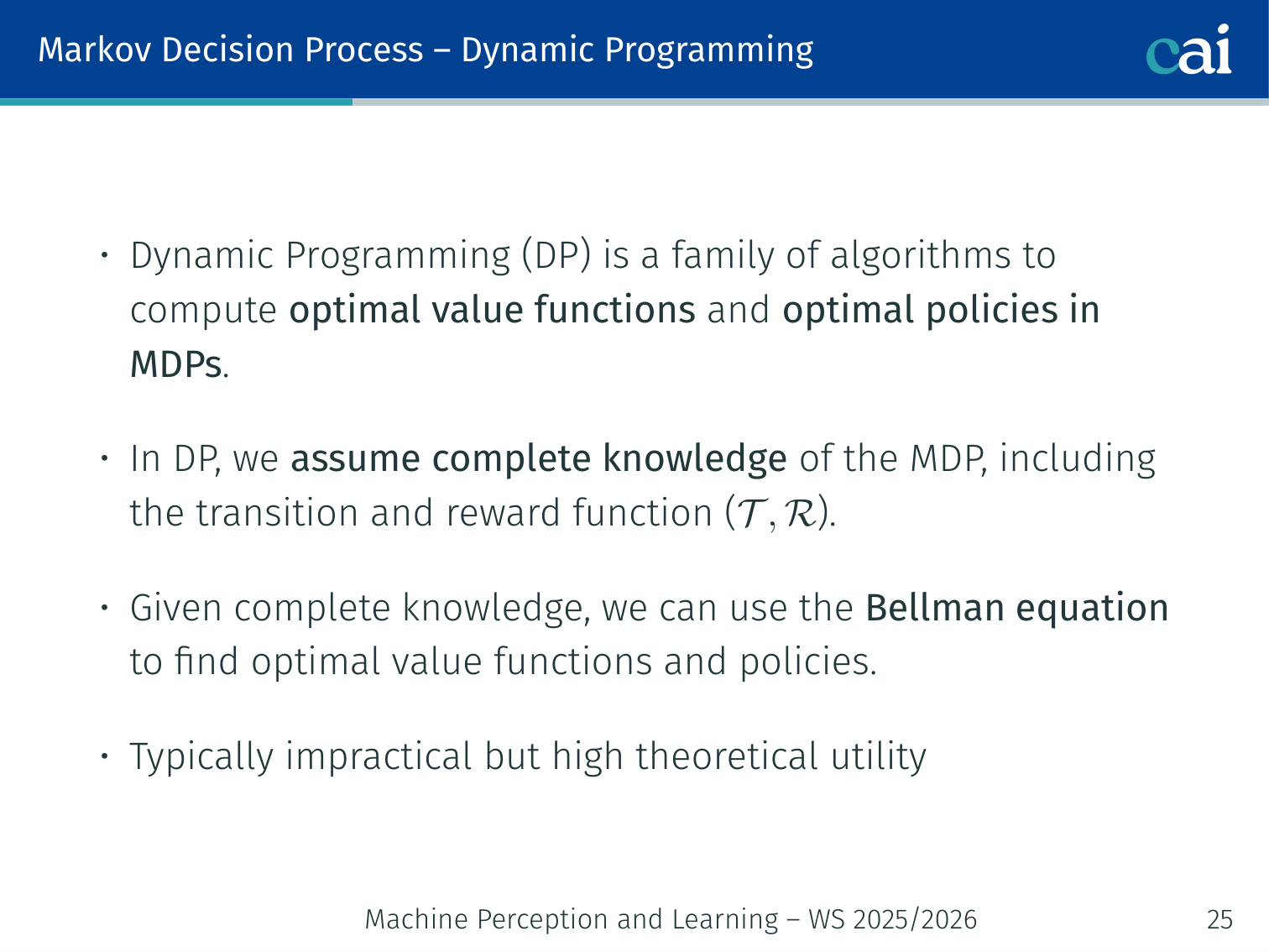
Using Dynamic Programming to solve MDPs when we know how the world works.

When the full model $(T,R)$ is known, we can find the optimal policy exactly.

Methods Overview

Method	Requires model?	How it works
Dynamic Programming	Yes	Iterate over all states using the model
Monte-Carlo	No	Full trajectory rollouts
Temporal-Difference	No	Bootstrap from visited states

Policy Iteration

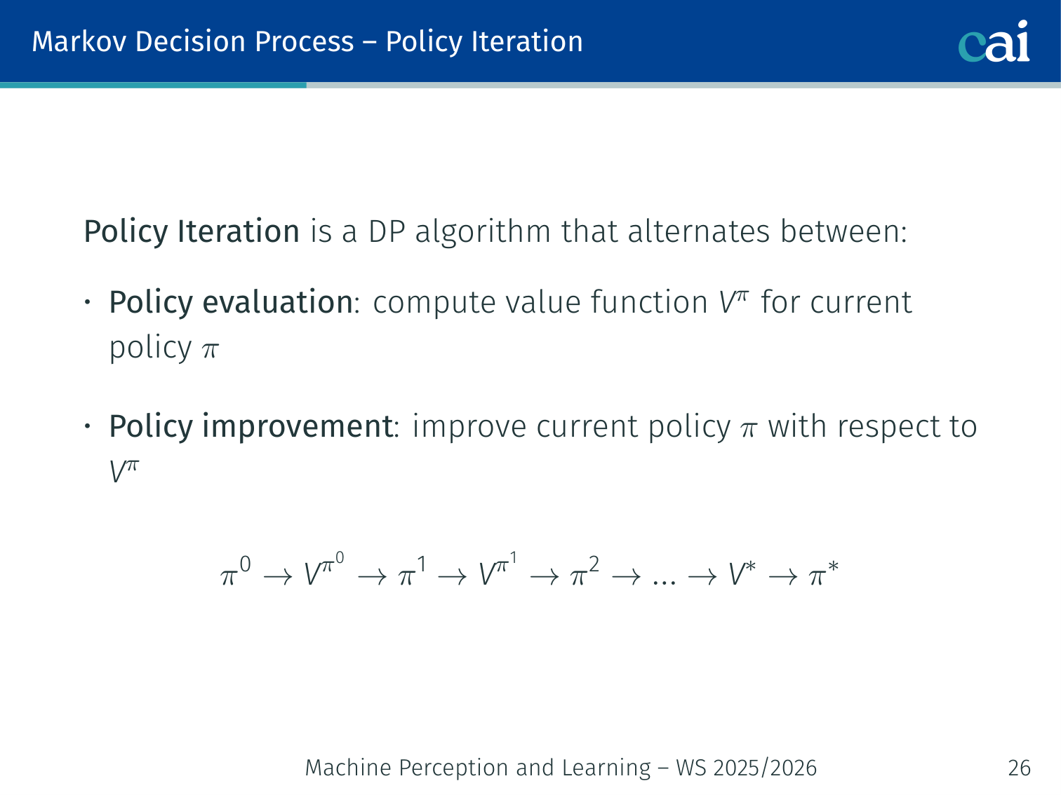
Policy Iteration: evaluating and then improving our policy step by step.

1. Policy Evaluation: compute $V^{\pi }$ for current $\pi$
2. Policy Improvement: update $\pi$ greedily w.r.t. $V^{\pi }$

${\pi }^0\stackrel{\text{eval}}{\to }{V}^{{\pi }^0}\stackrel{\text{improve}}{\to }{\pi }^1\to \dots \to V^{\ast }\to {\pi }^{\ast }$

Guaranteed to converge to ${\pi }^{\ast }$ in finite iterations.

Value Iteration

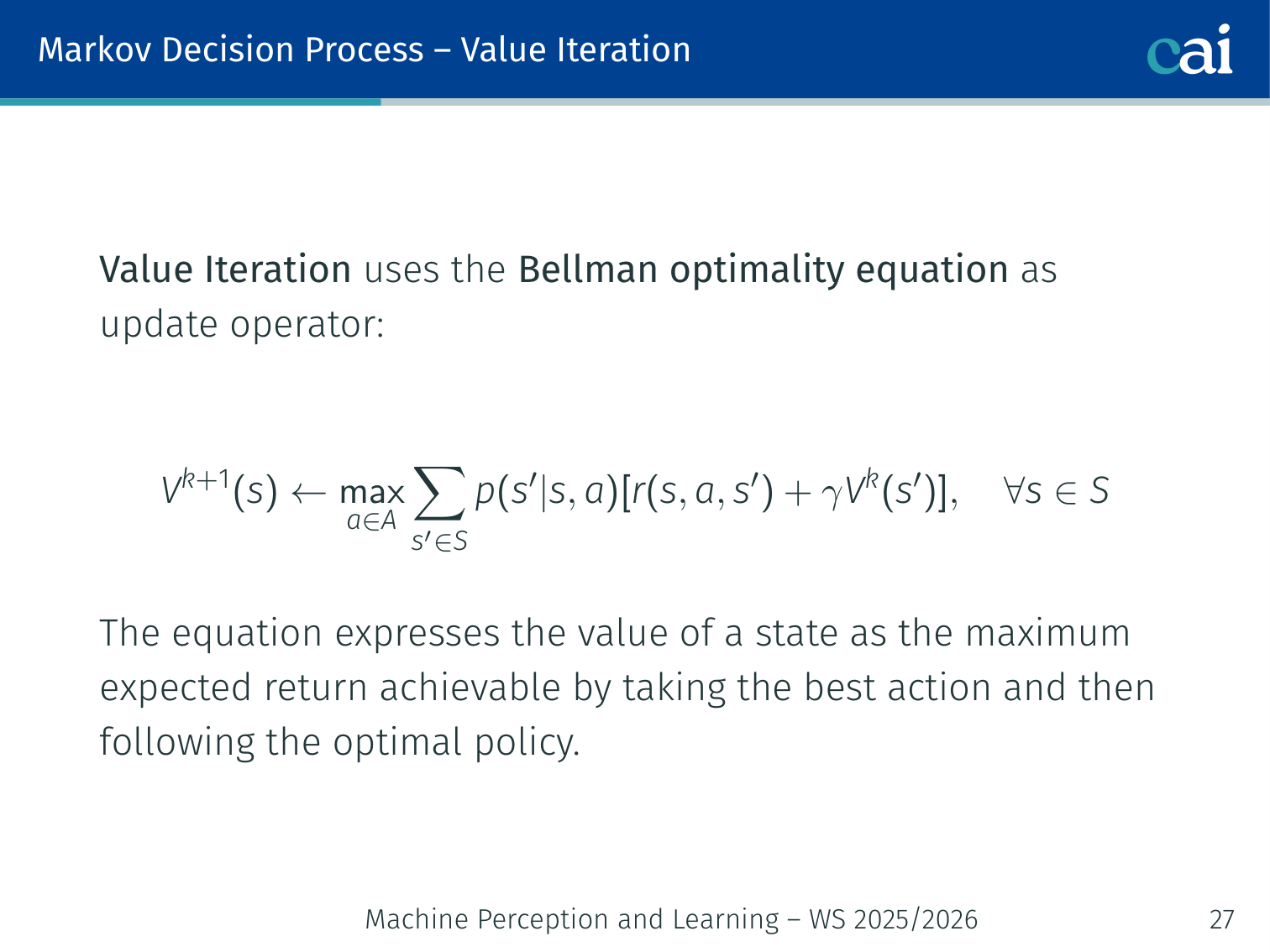
Value Iteration: searching for the best possible value function.

Apply the Bellman optimality equation as an update:

$V_{k+1}(s)\leftarrow {\max }_{a\in A}{\sum }_{s^{\prime }\in S}p(s^{\prime }|s,a)\left[r(s,a,s^{\prime })+\gamma V_k(s^{\prime })\right],\forall s\in S$

Algorithm:

Initialize V(s) = 0 for all s in S
repeat:
    for all s in S:
        V(s) <- max_{a} sum_{s'} p(s'|s,a) [r(s,a,s') + gamma*V(s')]
until V converged

pi*(s) = argmax_a sum_{s'} p(s'|s,a) [r(s,a,s') + gamma*V*(s')]

GridWorld Example ($\gamma =1$, step cost $=-5$)

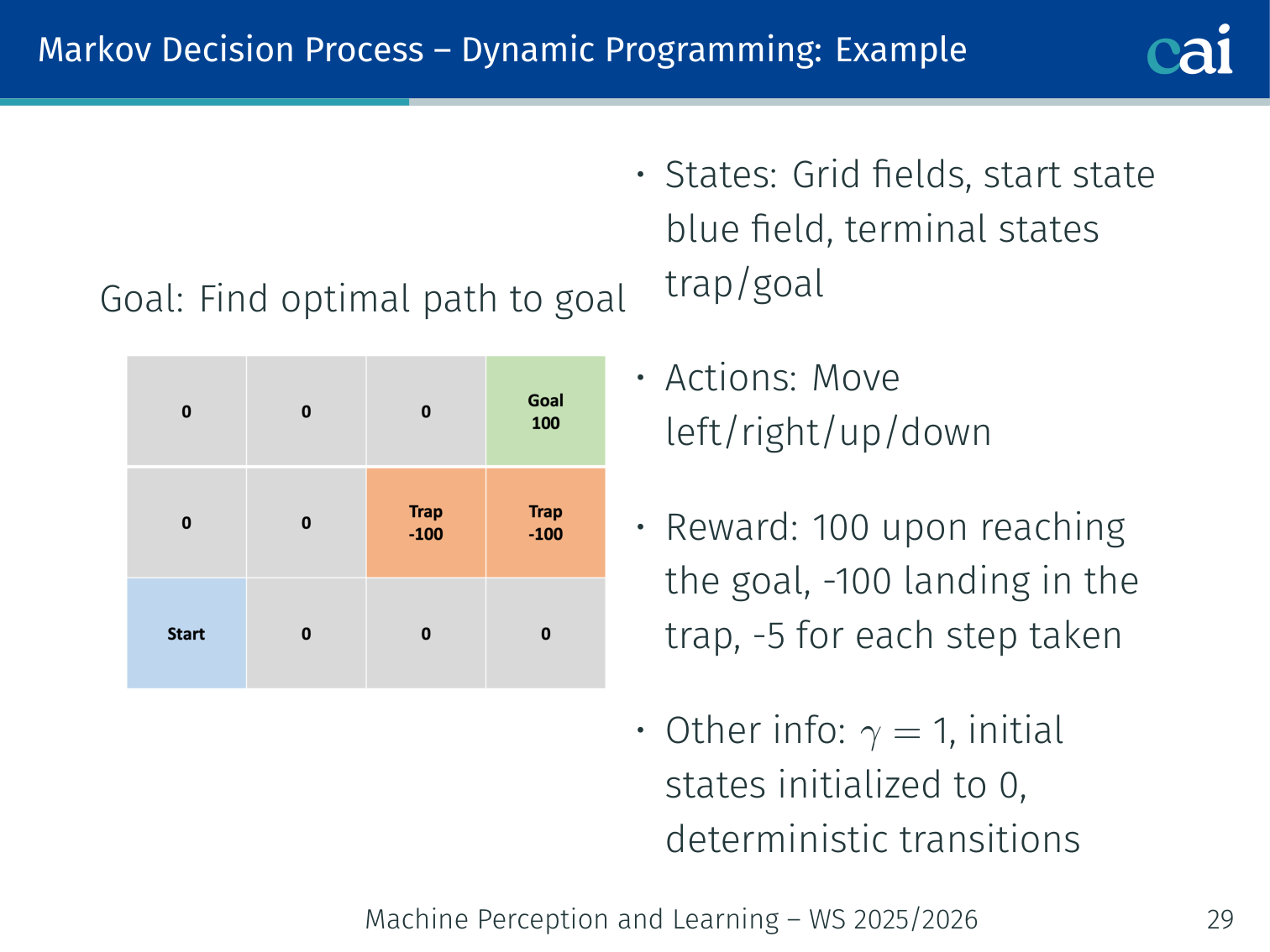
GridWorld: seeing how values propagate when every step has a cost.

4×4 grid: goal $+100$, trap $-100$, step cost $-5$. Deterministic transitions.

Iteration	Effect
0	All $V(s)=0$
1	Goal gets $+100$, trap gets $-100$. Adjacent cells update.
2–5	Values propagate outward from goal and trap.
6	Convergence — no further change. Greedy policy gives optimal path.

Intuition: value iteration “floods” the grid outward from the goal and trap. States close to the goal converge first; farther states feel the reward signal later.

Pros and Cons of Dynamic Programming

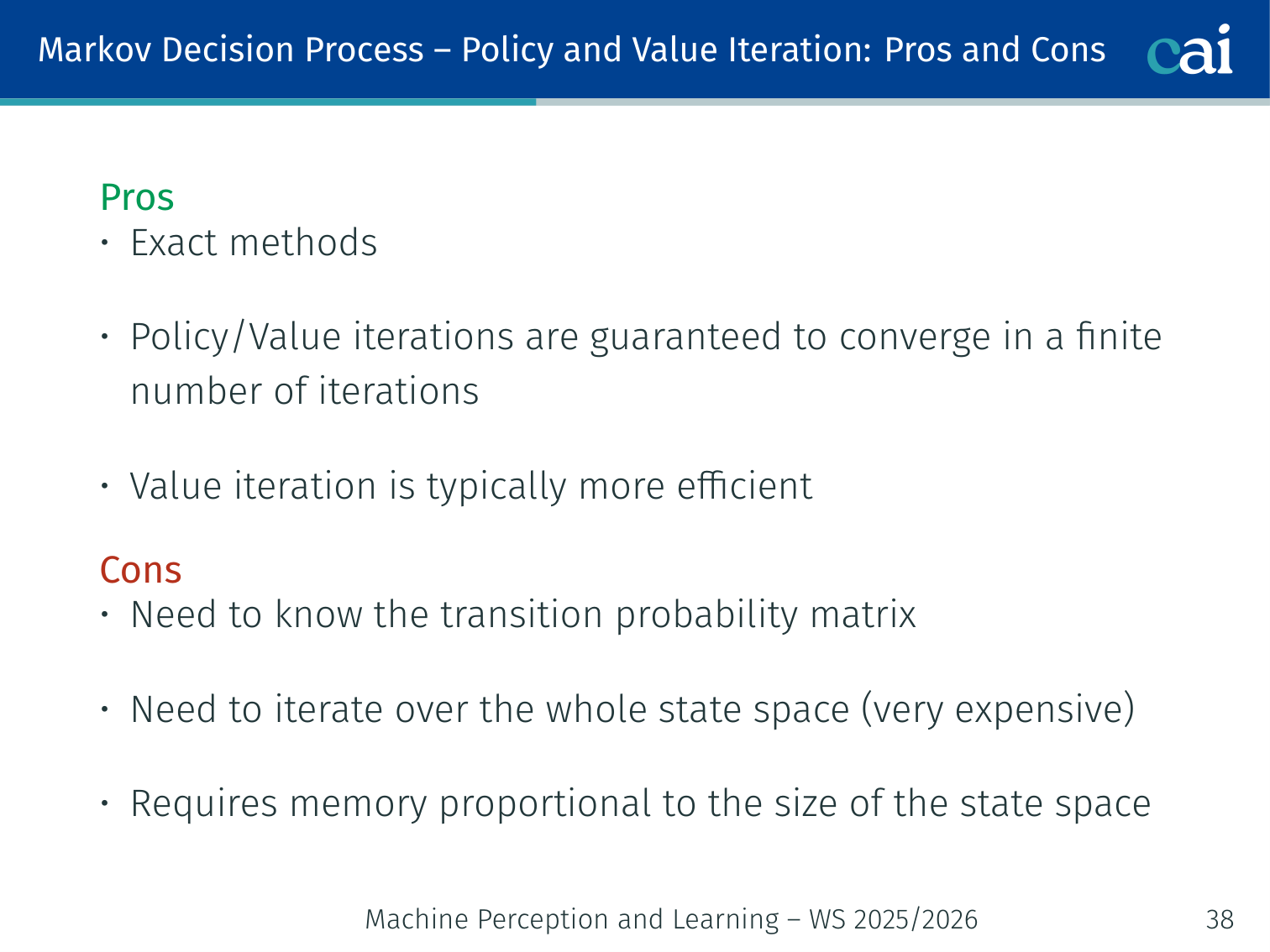
The pros and cons of using Dynamic Programming for RL.

✅ Exact — guaranteed convergence to ${\pi }^{\ast }$
✅ Value iteration more efficient than policy iteration
❌ Requires full model $p(s^{\prime }\mid s,a)$
❌ Must iterate over all $s\in S$ — infeasible for large/continuous spaces
❌ Memory proportional to $|S|$

When state space is too large → Temporal-Difference learning.

---

Temporal-Difference (TD) Learning

Core Idea

Only update visited states. Use bootstrapping: use current value estimates as targets without waiting for the episode to end.

For each step from $s$ via action $a$ to $s^{\prime }$: $\Delta V(s)=\underset{\text{TD target}}{\underbrace{r(s,a)+\gamma V(s^{\prime })}}-V(s)(\text{TD error})$ $V(s)\leftarrow V(s)+\alpha \Delta V(s),\alpha >0$

Exploration vs. Exploitation

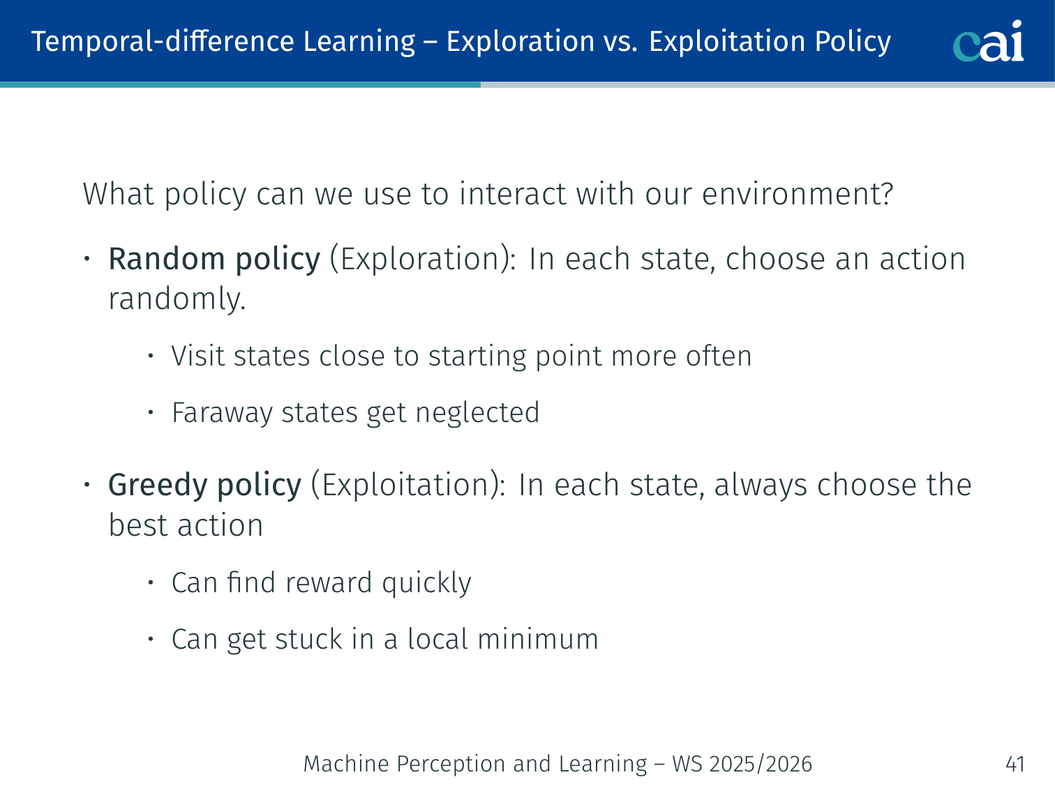
The exploration-exploitation tradeoff: trying new things vs. sticking to what works.

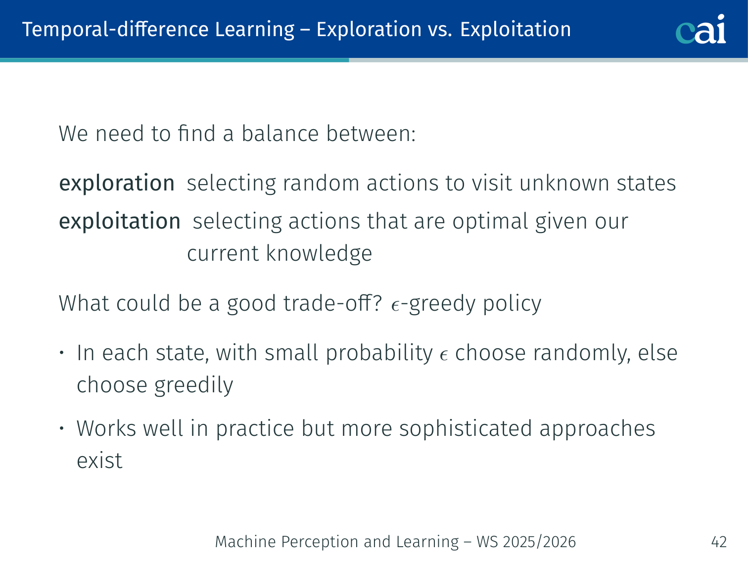
Exploration strategies: a look at how epsilon-greedy works.

Strategy	Description	Drawback
Random (pure exploration)	Choose randomly every step	Wastes effort on known bad states
Greedy (pure exploitation)	Always take highest-Q action	Gets stuck in local optima
$\epsilon$-greedy	Random with prob. $\epsilon$; greedy otherwise	Good practical balance

$\epsilon$ is typically annealed from $1.0$ down to a small value (e.g., $0.05$) over training.

Two Major Implementations

SARSA (On-Policy TD)

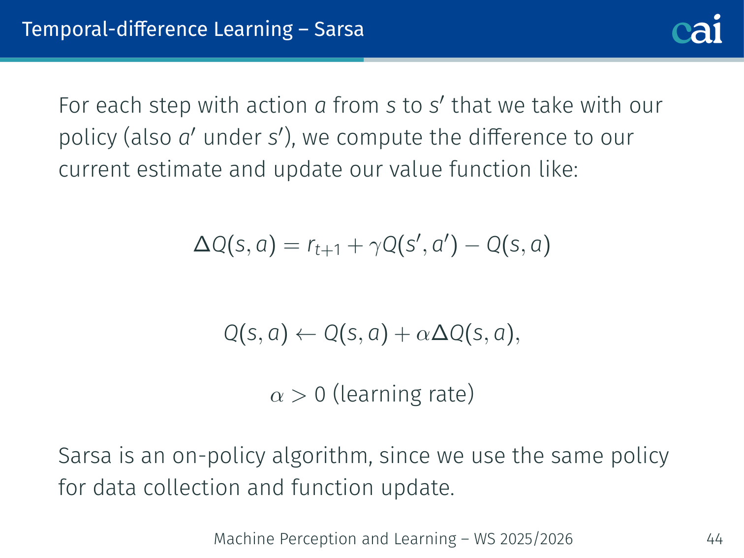
SARSA: a classic on-policy way to learn from temporal differences.

Uses the next action $a^{\prime }$ actually taken by the same policy:

$\Delta Q(s,a)=r_{t+1}+\gamma Q(s^{\prime },a^{\prime })-Q(s,a)$ $Q(s,a)\leftarrow Q(s,a)+\alpha \Delta Q(s,a)$

On-policy: the data-collection policy = the policy being updated. Because SARSA factors in the actual (possibly random) next action, it tends to be more cautious near dangerous states.

Example: Agent uses $\epsilon$-greedy. In state $s^{\prime }$ it randomly picks $a^{\prime }$. SARSA updates $Q$ using that random $a^{\prime }$, learning the value of the $\epsilon$-greedy policy itself — not the optimal one.

Q-Learning (Off-Policy TD)

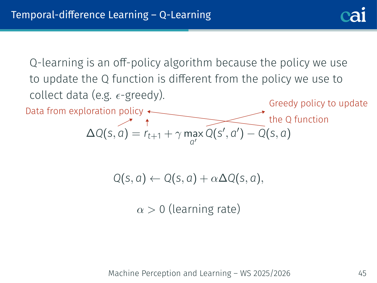
Q-Learning: the go-to off-policy method for TD learning.

Uses the best possible next action regardless of what the exploration policy would take:

$\Delta Q(s,a)=r_{t+1}+\gamma {\max }_{a^{\prime }}Q(s^{\prime },a^{\prime })-Q(s,a)$ $Q(s,a)\leftarrow Q(s,a)+\alpha \Delta Q(s,a)$

Off-policy: data collected via $\epsilon$-greedy, but updates use the greedy max — converges directly to $Q^{\ast }$.

💡 Intuition: SARSA Learns the Policy You Actually Use, Q-Learning Learns the Policy You Wish You Had

This is one of the most important conceptual splits in classical RL.

• SARSA asks: “given that I really do explore and sometimes make random moves, how good is this action?”
• Q-learning asks: “if I behave optimally from the next state onward, how good would this action be?”

That is why Q-learning is often more aggressive. It evaluates actions under the optimistic assumption that future choices will be greedy, while SARSA evaluates them under the actual exploratory behavior of the current policy.

SARSA vs. Q-Learning:

	SARSA	Q-Learning
Type	On-policy	Off-policy
Update target	$Q(s^{\prime },a^{\prime })$ — actual next action	${\max }_{a^{\prime }}Q(s^{\prime },a^{\prime })$ — best possible
Converges to	$Q^{\epsilon \text{-greedy}}$	$Q^{\ast }$
Risk behaviour	Cautious near danger	More aggressive during training

Worked Example: Q-Learning ($\gamma =1$, step cost $=0$, $\alpha =0.1$)

3x3 GridWorld. Goal at (2,2): reward +1. All Q = 0 initially.

Episode 1:
  s=(0,0), random "right" -> s'=(0,1), r=0
  DeltaQ = 0 + 1.0 * max Q(0,1,.) - 0 = 0   [no update yet]

Episode 2:
  ... -> s=(1,2) "down" -> s'=(2,2), r=+1  (goal!)
  DeltaQ[(1,2), down] = 1 + 0 - 0 = 1.0
  Q[(1,2), down] <- 0 + 0.1 * 1.0 = 0.1

Episode 3:
  s=(0,2) "down" -> s'=(1,2)
  DeltaQ[(0,2), down] = 0 + 1.0 * 0.1 - 0 = 0.1
  Q[(0,2), down] <- 0 + 0.1 * 0.1 = 0.01

After many episodes: Q-values converge; greedy policy traces shortest path to goal.

TD Learning: Pros and Cons

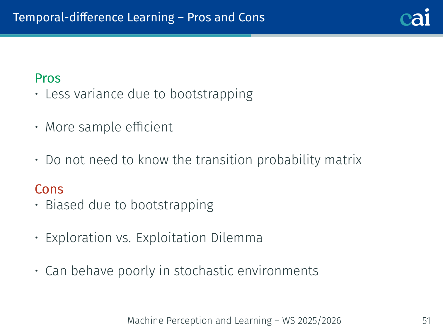
Weighing the pros and cons of TD learning methods.

✅ No model needed — does not require $p(s^{\prime }\mid s,a)$
✅ Online updates — learn after every step
✅ Lower variance than full Monte-Carlo
❌ Biased — bootstrapping introduces bias
❌ Exploration vs. exploitation dilemma
❌ Can behave poorly in stochastic environments

---

Deep Reinforcement Learning

Motivation: Tabular Methods Fail at Scale

• Learn each $(s,a)$ pair independently — no generalisation
• For raw image inputs (e.g., Atari frames), $|S|$ is astronomically large → Q-table impossible to store

Solution: approximate $Q(s,a)$ or $\pi (a|s)$ with a neural network.

---

Deep Q-Networks (DQN)

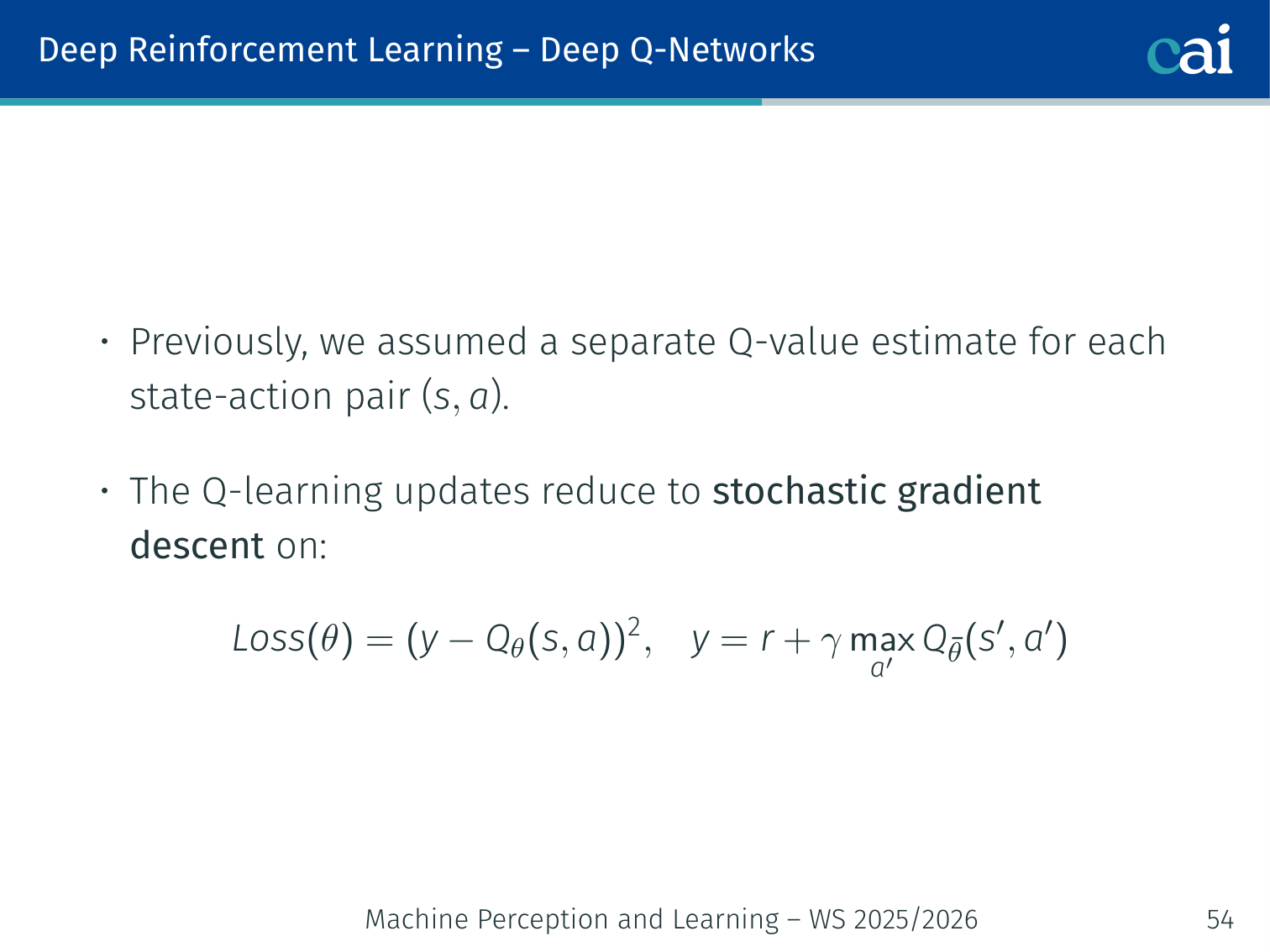
DQN: bringing the power of neural networks to Q-learning.

Use a neural network $Q_{\theta }(s,a)\approx Q^{\ast }(s,a)$. The Q-learning update becomes SGD on:

$\mathcal{L}(\theta )=\mathbb{E}\left[{\left(y-Q_{\theta }(s,a)\right)}^2\right],y=r+\gamma {\max }_{a^{\prime }}{Q}_{\bar{\theta }}(s^{\prime },a^{\prime })$

• $\bar{\theta }$ = target network (frozen copy of $\theta$, periodically synced for stability)

Experience Replay

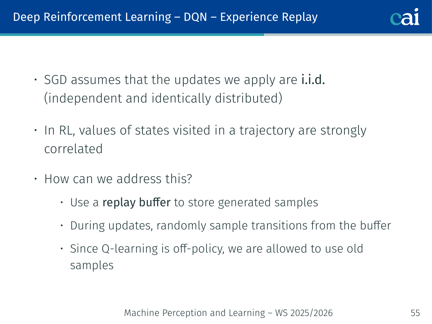
Experience Replay: how we break correlations to stabilize DQN training.

The replay buffer: sampling mini-batches to learn more efficiently.

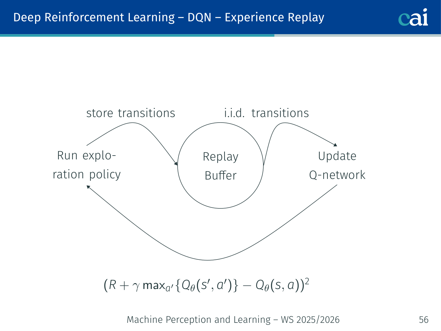
Problem: consecutive transitions are strongly correlated — violates SGD’s i.i.d. assumption.

Solution: store transitions in a replay buffer, sample random mini-batches for updates.

Run eps-greedy -> store (s, a, r, s') in Replay Buffer
                              |
                   Sample i.i.d. mini-batch
                              |
            Update Q-network via SGD on
        (r + gamma * max_{a'} Q_tbar(s',a') - Q_t(s,a))^2

Q-learning is off-policy → old buffer samples remain valid.

DQN Architecture (Atari)

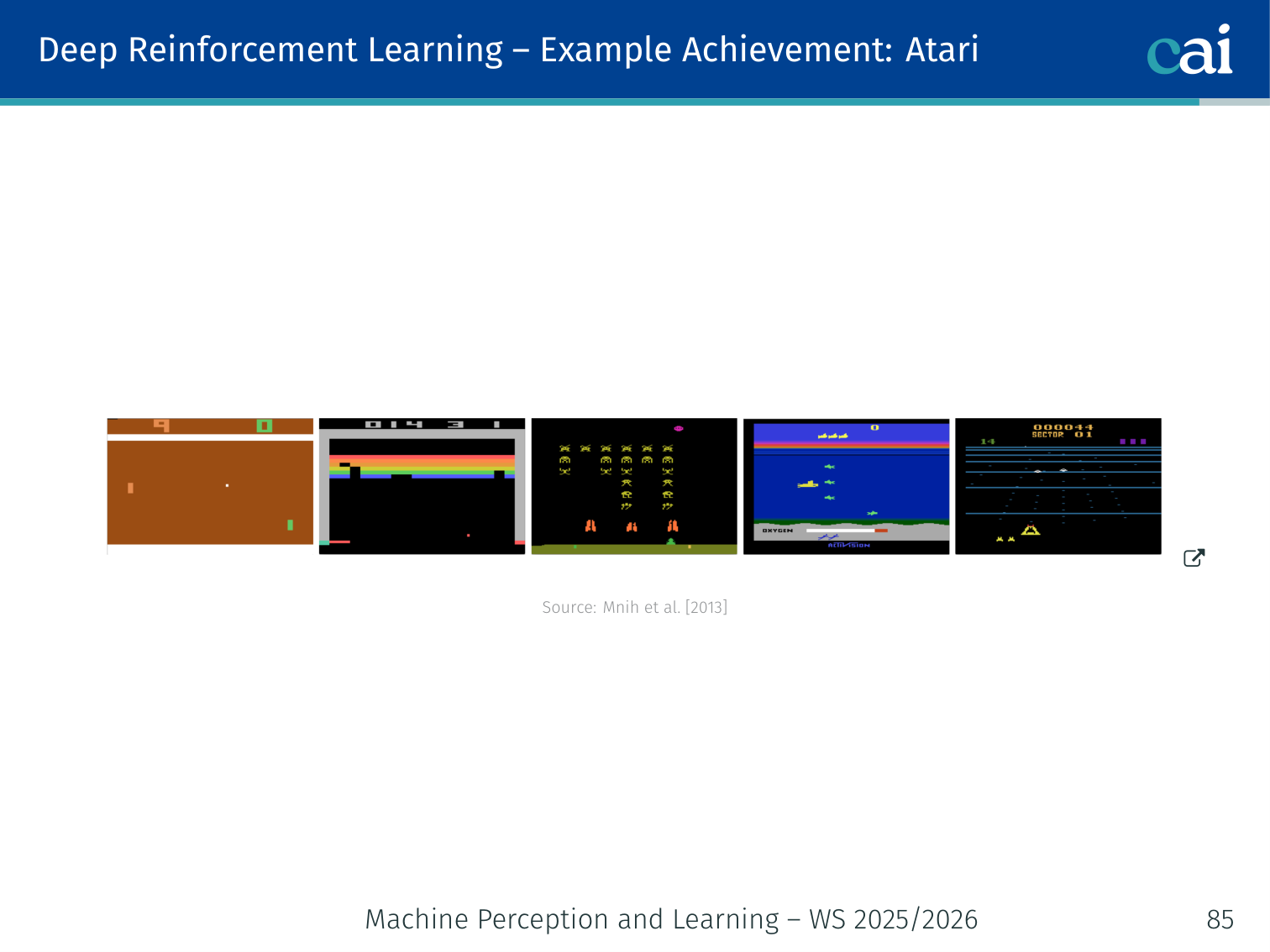
The DQN architecture that famously mastered Atari games.

Input: 4 stacked grayscale frames (84x84x4)
  -> Conv(8x8, 32 filters, stride=4) -> ReLU
  -> Conv(4x4, 64 filters, stride=2) -> ReLU
  -> Conv(3x3, 64 filters, stride=1) -> ReLU
  -> Flatten -> Dense(512) -> ReLU
  -> Dense(num_actions)    <- one Q-value per discrete action

Achievement: the DQN line of work showed that one architecture could learn directly from raw Atari pixels across many games. The widely cited superhuman Atari result is from the later Nature paper by Mnih et al. (2015).

DQN Key Tricks

A few essential tricks to keep DQN training from falling apart.

Trick	Why
Experience Replay	Break temporal correlations; reuse transitions efficiently
Target Network $Q_{\bar{\theta }}$	Stable training targets; prevent oscillations
ε-greedy	Balance exploration/exploitation during training

Limitation: DQN requires a discrete action space (one Q-value output per action).

---

Policy Gradient Methods

Policy Gradients: optimizing the policy directly instead of just values.

Instead of learning $Q$ and deriving $\pi$, directly optimise ${\pi }_{\theta }$ by gradient ascent on expected return.

Policy Evaluation

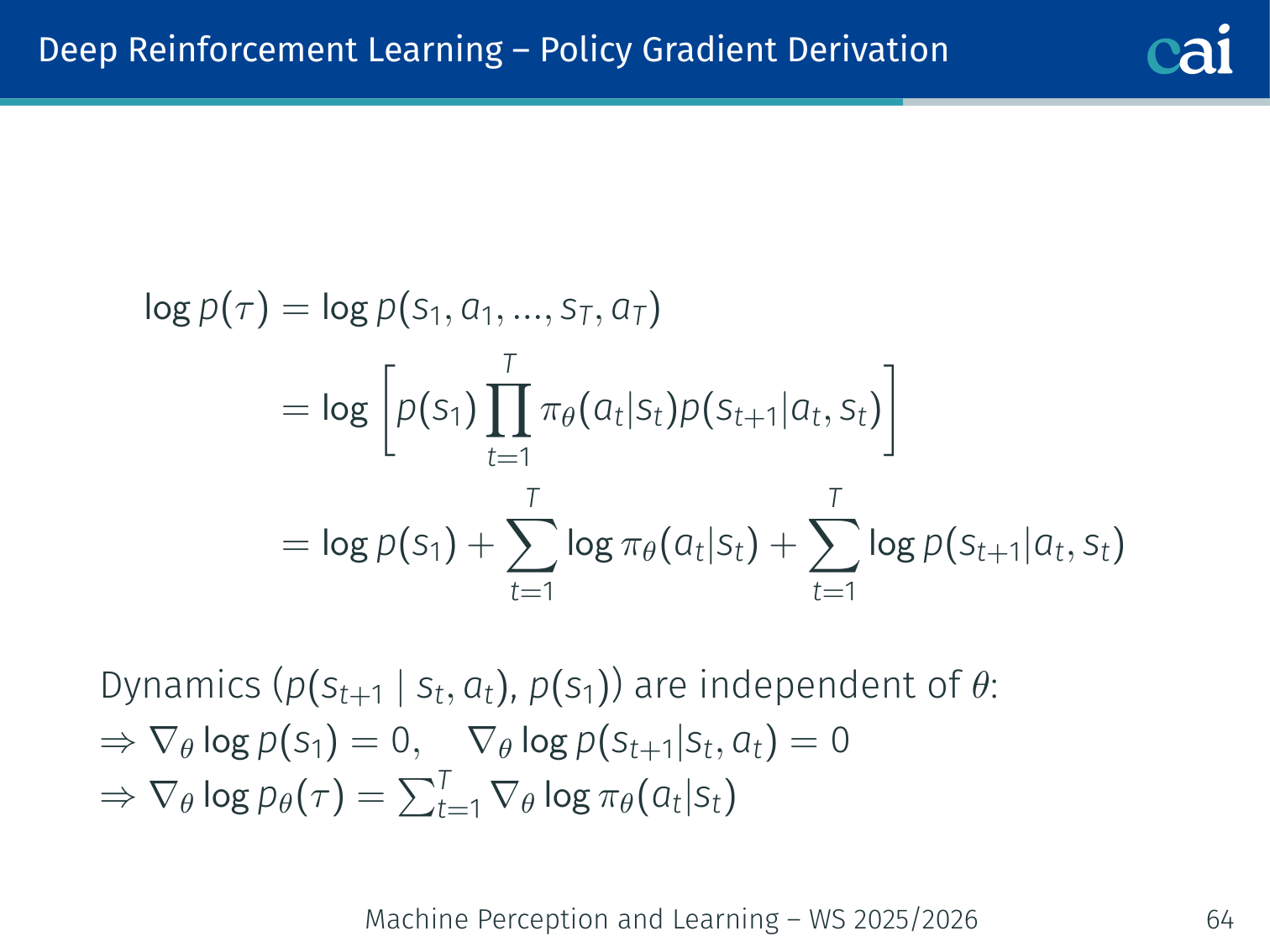
A trajectory $\tau =(s_1,a_1,\dots ,s_T,a_T)$ is sampled from:

$p_{\theta }(\tau )=p(s_1){\prod }_{t=1}^T{\pi }_{\theta }(a_t|s_t)p(s_{t+1}|a_t,s_t)$

Performance measure: $J(\theta )={\mathbb{E}}_{\tau \sim p_{\theta }(\tau )}\left[{\sum }_t{\gamma }^{t}r(s_t,a_t)\right]$

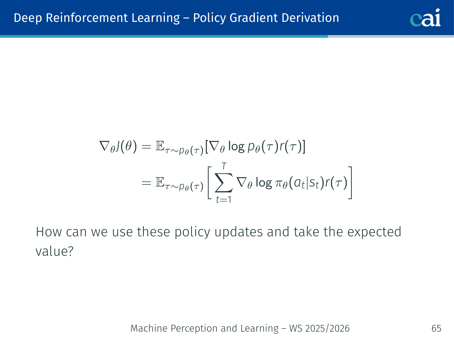
Objective: ${\theta }^{\ast }=\arg {\max }_{\theta }J(\theta )$, updated via $\theta \leftarrow \theta +{\nabla }_{\theta }J(\theta )$.

Policy Gradient Derivation

The log-probability trick: a key step in deriving policy gradients.

Wrapping up the derivation for the Policy Gradient theorem.

${\nabla }_{\theta }J(\theta )={\nabla }_{\theta }\int p_{\theta }(\tau )r(\tau )d\tau ={\mathbb{E}}_{\tau \sim p_{\theta }(\tau )}\left[{\nabla }_{\theta }\log p_{\theta }(\tau )r(\tau )\right]$

Since transition dynamics are independent of $\theta$: ${\nabla }_{\theta }\log p_{\theta }(\tau )={\sum }_{t=1}^T{\nabla }_{\theta }\log {\pi }_{\theta }(a_t|s_t)$

Policy gradient theorem: $\boxed{{\nabla }_{\theta }J(\theta )={\mathbb{E}}_{\tau \sim p_{\theta }(\tau )}\left[\sum _{t=1}^T{\nabla }_{\theta }\log {\pi }_{\theta }(a_t|s_t)\cdot r(\tau )\right]}$

Key property: no knowledge of environment dynamics needed — only the policy and sampled rewards.

💡 Intuition: Why the Log-Probability Trick Works

This update can look magical the first time you see it. In plain language, it says:

• if an action appeared in a high-return trajectory, increase its log-probability
• if it appeared in a low-return trajectory, decrease its log-probability

The term

${\nabla }_{\theta }\log {\pi }_{\theta }(a_t|s_t)$

points in the direction that would make action $a_t$ more likely in state $s_t$. Multiplying by return tells us whether that push should be positive or negative.

So policy gradients are basically weighted imitation of your own past behavior, where the weights come from how well that behavior turned out.

---

REINFORCE (Monte-Carlo Policy Gradient)

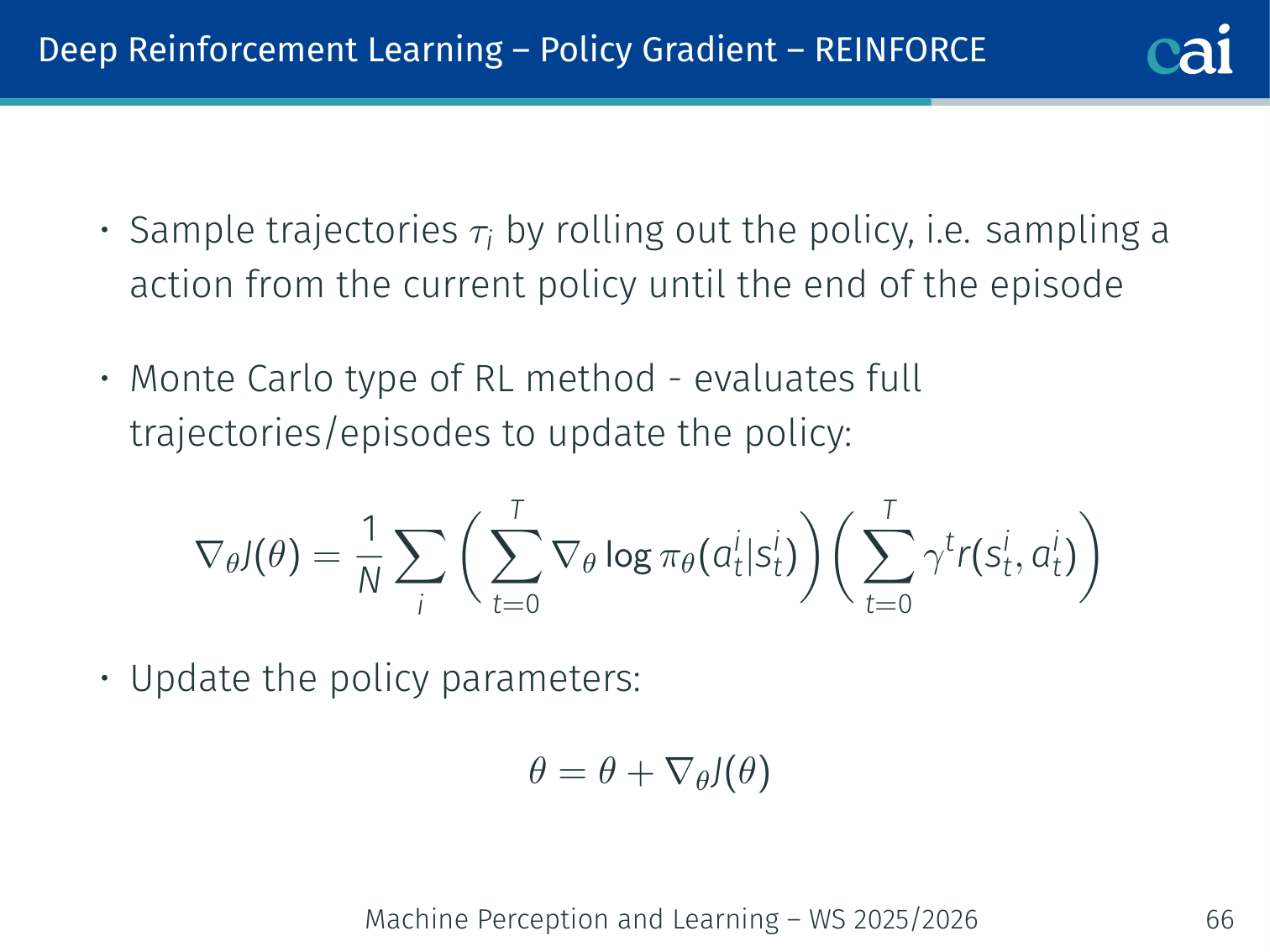
REINFORCE: using Monte-Carlo sampling to update our policy.

Sample $N$ full trajectory rollouts then update:

${\nabla }_{\theta }J(\theta )\approx \frac{1}{N}{\sum }_i\left({\sum }_{t=0}^T{\nabla }_{\theta }\log {\pi }_{\theta }(a_t^i|s_t^i)\right)\left({\sum }_{t=0}^T{\gamma }^{t}r(s_t^i,a_t^i)\right)$

$\theta \leftarrow \theta +\alpha {\nabla }_{\theta }J(\theta )$

Must complete full episodes before updating.

Intuition: high-return trajectories get their action probabilities boosted; bad ones are suppressed. “If it worked, do more of it.”

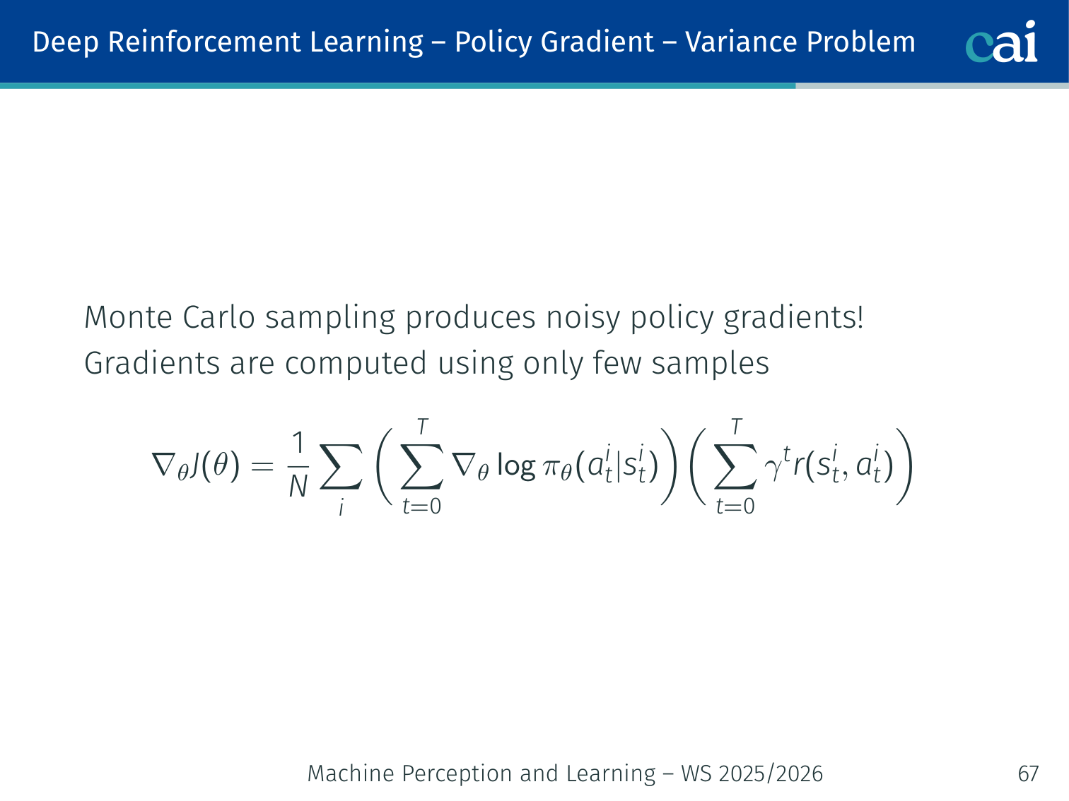
Variance Problem and Baseline

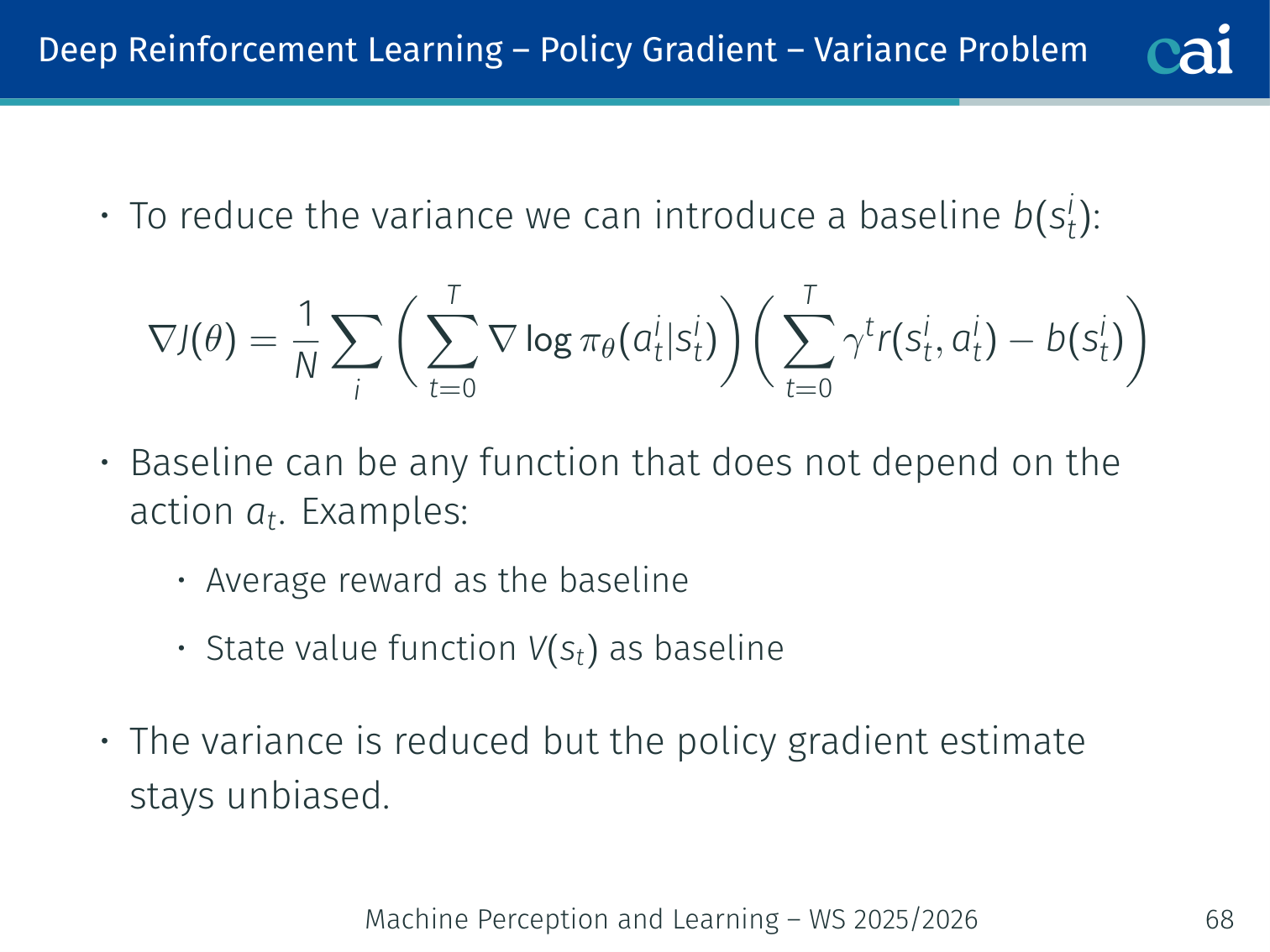
Using a baseline to keep policy gradient variance in check.

Subtracting a baseline: less noise, same unbiased gradient.

Monte-Carlo sampling → noisy gradients (few samples, high variance).

Fix: subtract a baseline $b(s_t)$ that is independent of $a_t$ (keeps gradient unbiased):

${\nabla }_{\theta }J(\theta )\approx \frac{1}{N}{\sum }_i{\sum }_t{\nabla }_{\theta }\log {\pi }_{\theta }(a_t^i|s_t^i)\left({\sum }_{t^{\prime }}{\gamma }^{t^{\prime }}{r}_{t^{\prime }}^i-b(s_t^i)\right)$

Common choices:

• Average reward across the batch
• State-value function $V(s_t)$ → advantage $A_t=G_t-V(s_t)$

---

Actor-Critic

Actor-Critic: combining policy (actor) and value (critic) estimation.

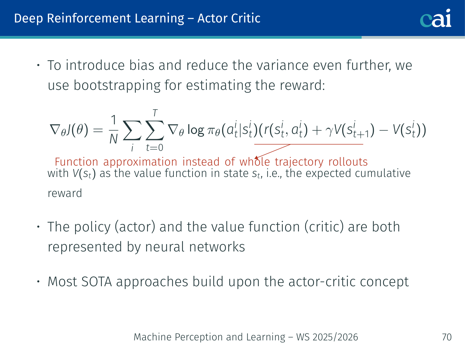
Using TD error to estimate the "advantage" in Actor-Critic.

Reduce variance further (with some bias) by using bootstrapping instead of full returns:

${\nabla }_{\theta }J(\theta )\approx \frac{1}{N}{\sum }_i{\sum }_t{\nabla }_{\theta }\log {\pi }_{\theta }(a_t^i|s_t^i)\underset{{\hat{A}}_t=\text{ estimated advantage (TD error)}}{\underbrace{(r(s_t^i,a_t^i)+\gamma V(s_{t+1}^i)-V(s_t^i))}}$

This is the advantage function with a bootstrapped estimate: $A_t=Q(s_t,a_t)-V(s_t)\approx r(s_t,a_t)+\gamma V(s_{t+1})-V(s_t)={\hat{A}}_t$

Architecture:

        State s
          |
   +------+------+
   |             |
 Actor         Critic
(pi_theta)    (V_phi)
 a ~ pi(.|s)   V(s)  ->  compute A_hat_t

• Actor: policy network ${\pi }_{\theta }$, updated by gradient ascent using ${\hat{A}}_t$
• Critic: value network $V_{\varphi }$, updated by minimising $(r+\gamma V(s^{\prime })-V(s){)}^2$

Most SOTA RL algorithms build on actor-critic.

💡 Intuition: Actor-Critic Splits “What To Do” From “How Good It Was”

Actor-critic is easier to remember if you personify the two parts:

• Actor = the decision-maker
• Critic = the evaluator

The actor proposes actions. The critic estimates whether the current situation is better or worse than expected. The TD error then becomes a training signal saying:

• “that action turned out better than expected, do more of it”
• or “that action turned out worse than expected, do less of it”

This split is powerful because it keeps the policy update low-variance without forcing the policy to learn everything from raw returns alone.

---

Why Vanilla Actor-Critic is Fragile

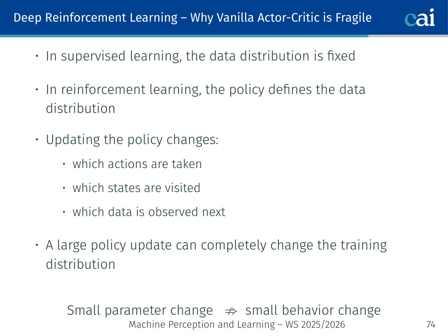
Why basic Actor-Critic can be so fragile and unstable.

In supervised learning: data distribution is fixed.

In RL: the policy defines the data distribution:

• A policy update changes which actions are taken → which states are visited → which data is seen next

Small parameter change ⟹ potentially huge behaviour change

A single large update can completely collapse the training distribution.

---

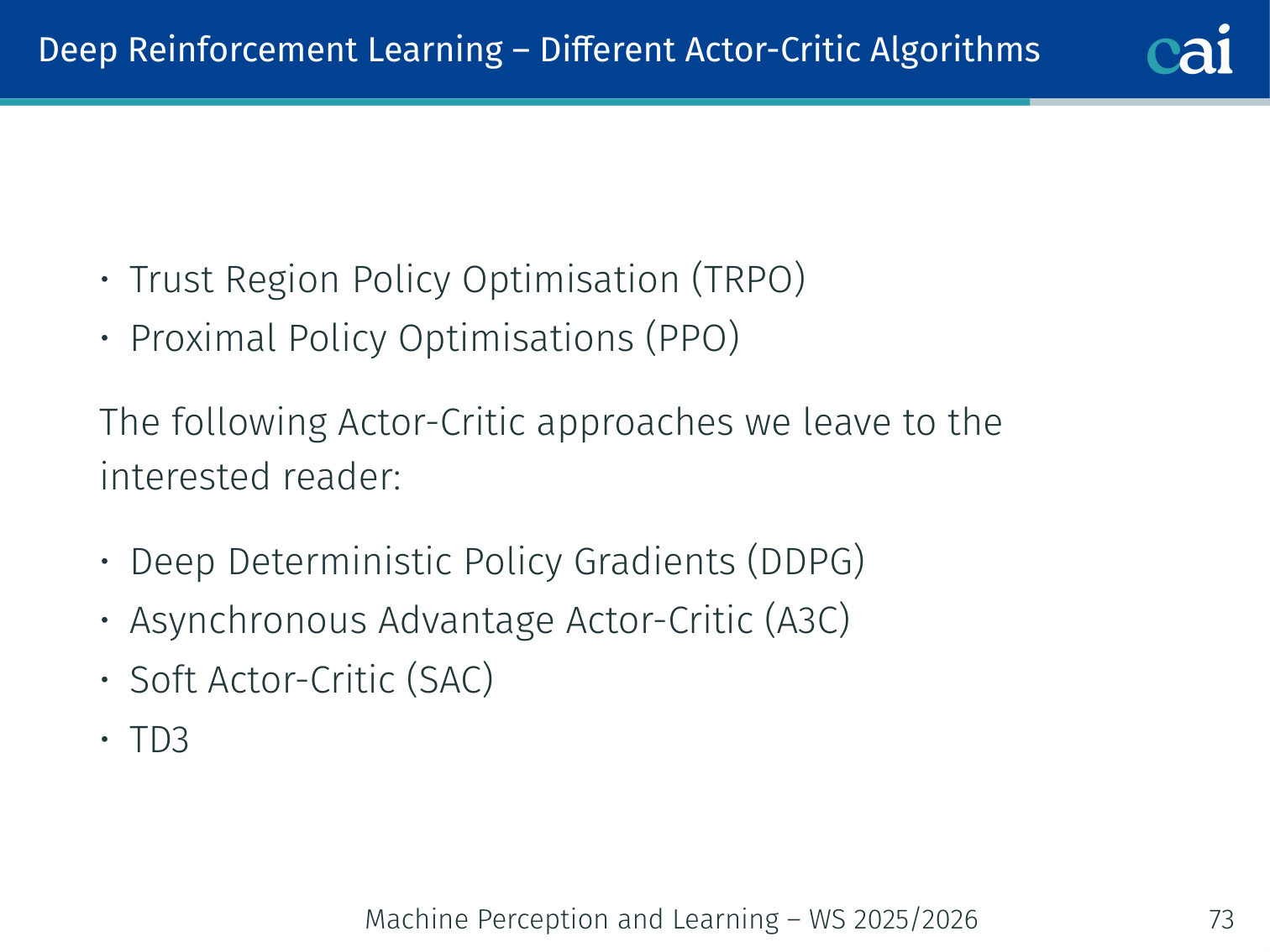
Trust Region Policy Optimisation (TRPO)

TRPO: making policy updates more stable by staying in a "trust region".

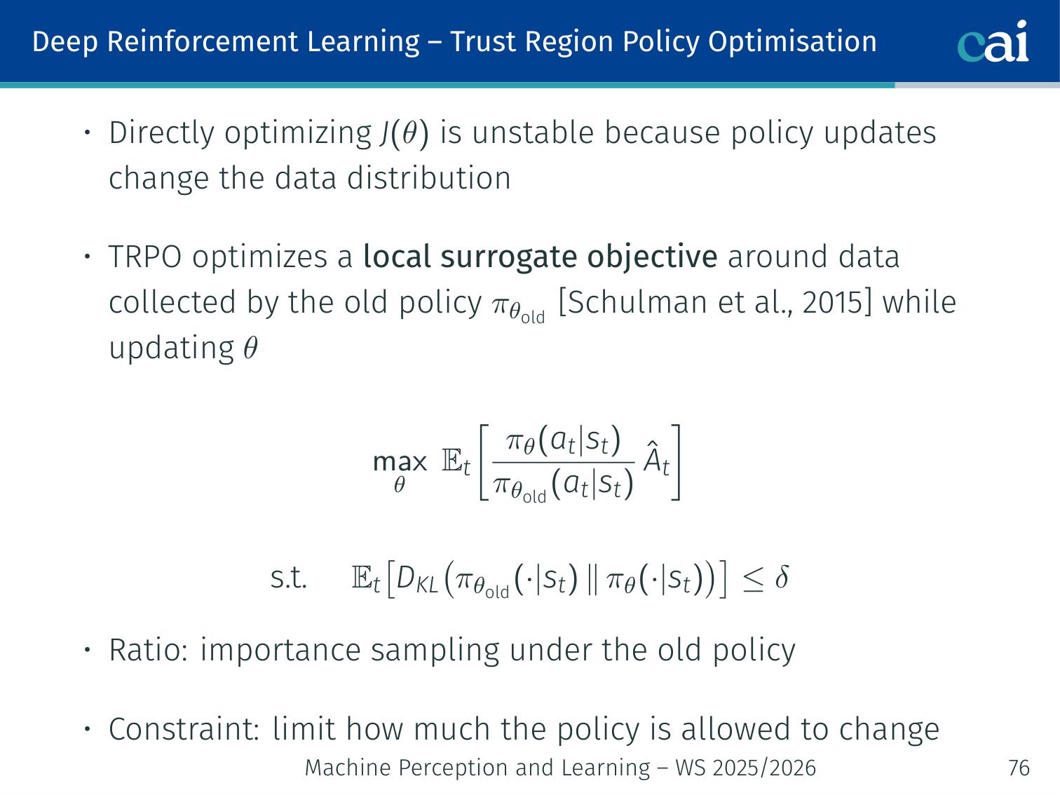
Constraining KL divergence to keep policy updates from going off the rails.

Step size is much harder to tune in RL than in SL:

• Too small → slow learning
• Too large → catastrophic collapse

TRPO [Schulman et al., 2015]: optimise a surrogate objective using old-policy data, constrained by a hard KL divergence limit:

${\max }_{\theta }{\mathbb{E}}_t\left[\frac{{\pi }_{\theta }(a_t|s_t)}{{\pi }_{{\theta }_{\text{old}}}(a_t|s_t)}{\hat{A}}_t\right]\text{s.t.}{\mathbb{E}}_t\left[D_{\text{KL}}\left({\pi }_{{\theta }_{\text{old}}}(\cdot |s_t)\Vert {\pi }_{\theta }(\cdot |s_t)\right)\right]\le \delta$

• Probability ratio: importance sampling correction for using old-policy data
• KL constraint: keeps the update inside a “trust region”
• Solved via Fisher Information Matrix + conjugate gradient — second-order method (expensive)

---

Proximal Policy Optimisation (PPO)

PPO: a much simpler and more popular alternative to TRPO.

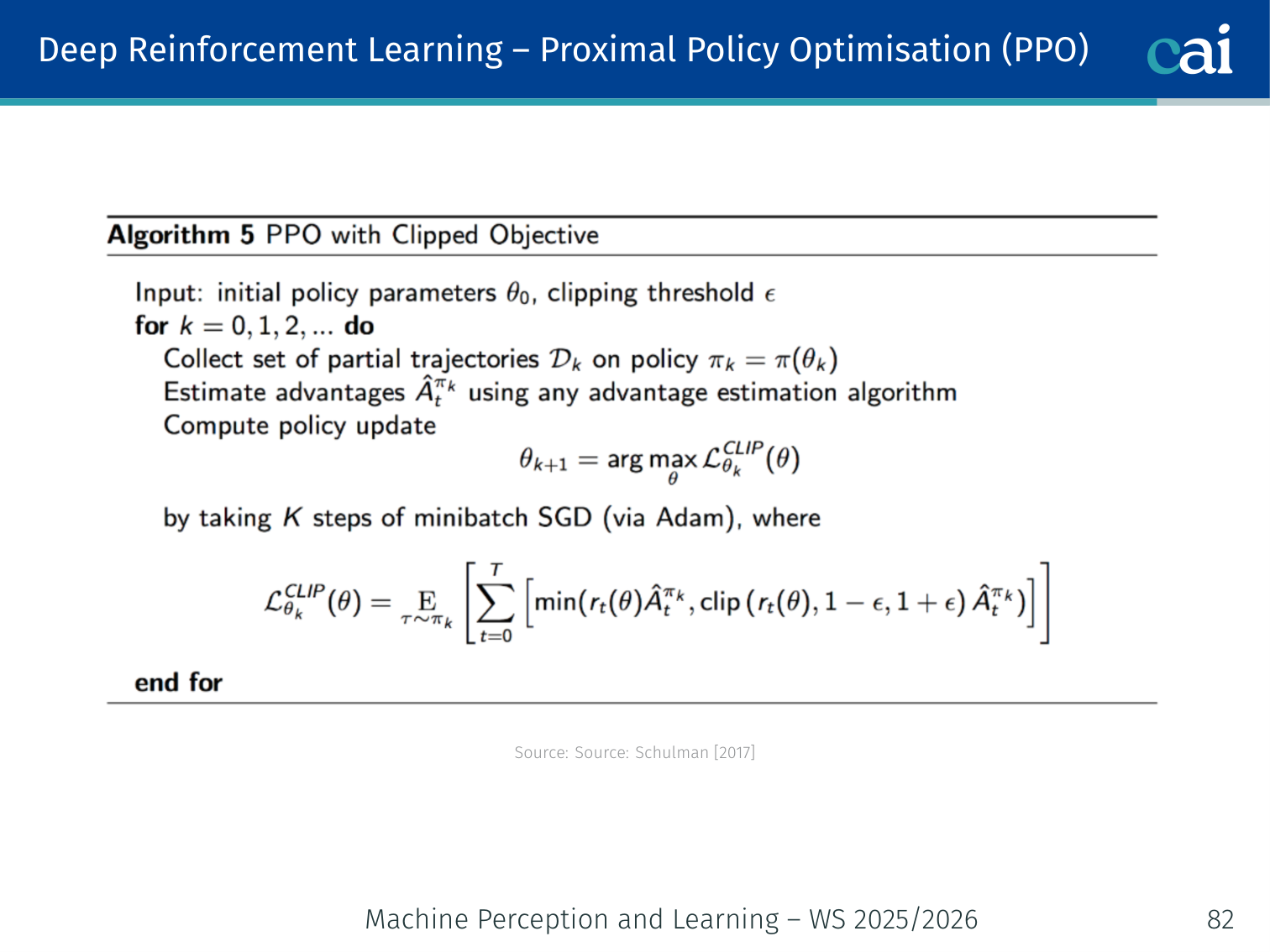
PPO [Schulman et al., 2017]: the practical successor to TRPO.

Step 1: KL Penalty (Soft Constraint)

Replace the hard constraint with a tunable penalty:

${\max }_{\theta }{\mathbb{E}}_t\left[\frac{{\pi }_{\theta }(a_t|s_t)}{{\pi }_{{\theta }_{\text{old}}}(a_t|s_t)}{\hat{A}}_t\right]-\beta \cdot {\mathbb{E}}_t\left[D_{\text{KL}}\left({\pi }_{{\theta }_{\text{old}}}(\cdot |s_t)\Vert {\pi }_{\theta }(\cdot |s_t)\right)\right]$

Step 2: Clipped Objective (PPO-CLIP) — the standard version

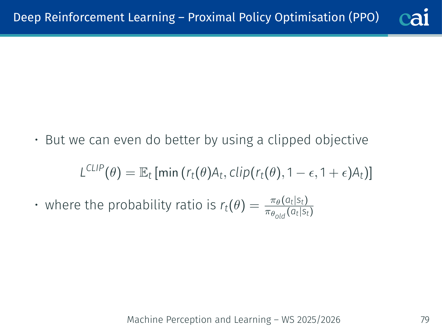
PPO-CLIP: clipping the objective to prevent those dangerous large updates.

Clip the probability ratio directly:

${\mathcal{L}}^{\text{CLIP}}(\theta )={\mathbb{E}}_t\left[\min \left(r_t(\theta ){\hat{A}}_t,\mathrm{clip}(r_t(\theta ),1-\epsilon ,1+\epsilon ){\hat{A}}_t\right)\right]$

where $r_t(\theta )=\frac{{\pi }_{\theta }(a_t|s_t)}{{\pi }_{{\theta }_{\text{old}}}(a_t|s_t)}$

Clipping mechanics (typical $\epsilon =0.2$, clip range $[0.8,1.2]$):

Scenario	Effect
${\hat{A}}_t>0$, $r_t>1.2$	Clipped — no further incentive to push it higher
${\hat{A}}_t>0$, $r_t\in [0.8,1.2]$	Normal gradient ascent
${\hat{A}}_t<0$, $r_t<0.8$	Clipped — no further incentive to push it lower
${\hat{A}}_t<0$, $r_t\in [0.8,1.2]$	Normal gradient descent

Intuition: The $\min$ ensures the objective stops rewarding changes once the ratio moves too far outside $[1-\epsilon ,1+\epsilon ]$ in the helpful direction.

🧠 Deep Dive: Why PPO Can Reuse the Same Batch for Multiple Epochs

Vanilla policy gradient is fragile because once the policy changes, old samples quickly become stale.

PPO’s ratio

$r_t(\theta )=\frac{{\pi }_{\theta }(a_t|s_t)}{{\pi }_{{\theta }_{\text{old}}}(a_t|s_t)}$

explicitly tracks how far the new policy has moved away from the policy that generated the data.

That does two useful things:

• it lets us still learn from trajectories collected by the old policy
• clipping prevents us from exploiting that old data too aggressively

This is why the original PPO paper emphasizes that the method supports multiple epochs of minibatch updates on the same sampled batch while remaining much simpler than TRPO.

Worked Example ($\epsilon =0.2$):

Action a in state s, advantage A_hat = +2.0 (good action)
  pi_old(a|s) = 0.30
  pi_new(a|s) = 0.45  ->  ratio = 0.45/0.30 = 1.50

  Without clipping:  L = 1.50 * 2.0 = 3.0
  With clip(1.50, 0.8, 1.2) = 1.2:
    L = min(1.50*2.0, 1.2*2.0) = min(3.0, 2.4) = 2.4

  Update is capped — cannot become too aggressive even for a very good action.

PPO vs. TRPO

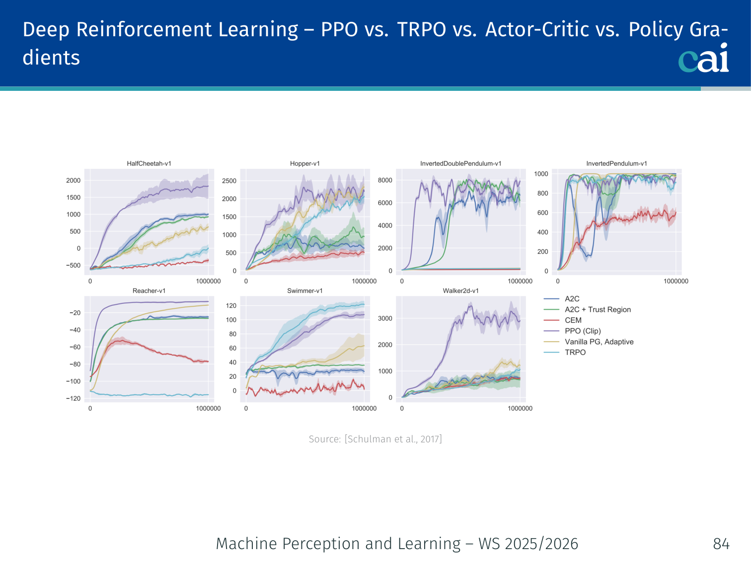
PPO vs. TRPO: weighing performance against complexity.

Property	TRPO	PPO
Constraint	Hard KL	Clipped ratio
Optimisation order	Second-order (conjugate gradient)	First-order (Adam)
Implementation complexity	High	Low
Computation cost	Heavy	Lightweight
Performance	Good	Comparable or better

---

Reinforcement Learning from Human Feedback (RLHF)

Large language models are initially trained with next-token prediction, which teaches them to model text distributions well. But this objective does not directly optimise for what humans actually want: helpfulness, harmlessness, honesty, instruction-following, or style preferences. RLHF addresses this gap by turning human preferences into a learning signal (Ouyang et al., 2022).

Three-Stage Pipeline

1. Supervised Fine-Tuning (SFT)

Start from a pre-trained language model and fine-tune it on human-written demonstrations of good behaviour.

• Input: prompt $x$
• Target: high-quality human response $y$
• Result: a model that can follow instructions reasonably well

2. Reward Model Training

Next, collect human preference comparisons. Annotators are shown two candidate responses for the same prompt and choose the better one.

If $y_w$ is the preferred response and $y_l$ the rejected one, the reward model $r_{\varphi }$ is trained so that

$$r_{\varphi }(x,y_w)>r_{\varphi }(x,y_l)$$

A common pairwise objective is

$${\mathcal{L}}_{\text{RM}}=-\log \sigma \left(r_{\varphi }(x,y_w)-r_{\varphi }(x,y_l)\right)$$

so the reward model learns to approximate human preference.

3. RL Fine-Tuning with PPO

Finally, optimise the policy against the reward model using PPO. The objective is not just “maximise reward”, but “maximise reward while staying close to the reference model”:

$$\underset{\theta }{\max }{\mathbb{E}}_{y\sim {\pi }_{\theta }(\cdot |x)}\left[r_{\varphi }(x,y)\right]-\beta D_{\text{KL}}\left({\pi }_{\theta }(\cdot |x)\Vert {\pi }_{\text{ref}}(\cdot |x)\right)$$

where:

• ${\pi }_{\theta }$ is the current policy
• ${\pi }_{\text{ref}}$ is usually the SFT model
• $r_{\varphi }$ is the learned reward model
• $\beta$ controls how strongly we penalise deviation from the reference model

Why the KL Penalty Matters

Without the KL term, the model may exploit weaknesses in the reward model and drift toward unnatural text. This is a form of reward hacking.

The KL penalty helps because it:

• keeps the policy close to the original language model
• preserves fluency and general language competence
• prevents the model from chasing spurious high-reward behaviours too aggressively

Example: A reward model might accidentally prefer overly long, overly flattering, or repetitive answers. Without a KL penalty, the policy could exploit this artifact instead of becoming genuinely more helpful.

🧠 Deep Dive: Why RLHF Uses a Per-Token KL “Leash”

In the InstructGPT setup, OpenAI explicitly adds a per-token KL penalty from the SFT model during PPO to reduce over-optimization of the reward model.

That is a very practical design choice. The reward model is only an approximation of human preference, so if the policy is allowed to optimize it too hard, it may discover weird hacks that score well but sound unnatural.

A helpful intuition is to think of the KL term as a leash:

• the reward model pulls the policy toward preferred behavior
• the KL term pulls it back toward the fluent, general-purpose SFT model

Good RLHF needs both forces. If reward dominates completely, the model can become brittle and exploitative. If KL dominates completely, the model barely changes and alignment gains are weak.

RLHF in One Picture

Stage	Data source	Objective
SFT	Human demonstrations	Learn to imitate good answers
Reward model	Human preference comparisons	Learn a scalar proxy for human judgement
RL with PPO	Model-generated responses + reward model	Optimise policy while constraining KL drift

In short, RLHF combines supervised learning, preference modelling, and reinforcement learning. In practice, the RL stage is usually performed with PPO, which is why PPO became central to instruction-tuning pipelines such as InstructGPT (Ouyang et al., 2022).

PyTorch Implementation: Proximal Policy Optimization (PPO)

A quick look at how to implement PPO in PyTorch.

PPO is an actor-critic algorithm that ensures stable training by limiting how much the policy can change in a single update.

import torch
import torch.nn as nn
from torch.distributions import Categorical
 
# 1. The Actor-Critic Network
class ActorCritic(nn.Module):
    def __init__(self, state_dim, action_dim):
        super().__init__()
 
        # --- THE ACTOR (Policy) ---
        # Input: State features
        # Output: Probability distribution over actions
        self.actor = nn.Sequential(
            nn.Linear(state_dim, 64),
            nn.Tanh(), # Tanh is common in RL for smooth gradients
            nn.Linear(64, action_dim),
            nn.Softmax(dim=-1) # Ensures action probabilities sum to 1
        )
 
        # --- THE CRITIC (Value Function) ---
        # Input: State features
        # Output: A single scalar V(s) representing expected future reward
        self.critic = nn.Sequential(
            nn.Linear(state_dim, 64),
            nn.Tanh(),
            nn.Linear(64, 1)
        )
 
    def act(self, state):
        """Used during data collection to pick actions."""
        probs = self.actor(state)
        # Categorical distribution handles sampling and log-probs for us
        dist = Categorical(probs)
        action = dist.sample() # Sample action according to policy
        return action, dist.log_prob(action)
 
    def evaluate(self, state, action):
        """Used during the update step to evaluate taken actions."""
        probs = self.actor(state)
        dist = Categorical(probs)
 
        action_logprobs = dist.log_prob(action)
        dist_entropy = dist.entropy() # Entropy encourages exploration
        state_value = self.critic(state) # V(s)
 
        return action_logprobs, state_value, dist_entropy

Key RL Concepts:

• The Actor-Critic Split: The Actor focuses on behavior (what to do), while the Critic focuses on judgment (how good the current state is).
• Log-Probabilities: In RL, we maximize the log-probability of actions that led to high rewards.
• Entropy: High entropy means the policy is “uncertain” and spread out, which is good for exploring different actions. PPO often adds an entropy bonus to the loss to prevent the model from becoming too greedy too early.

---

Notable Achievements

Achievement	Algorithm	Reference
Atari at superhuman level from raw pixels	DQN	Mnih et al., 2015
Mastering the game of Go	AlphaGo (policy/value net + MCTS)	Silver et al., 2016
Locomotion and continuous control	PPO / TRPO	Schulman et al., 2017
Grandmaster StarCraft II	AlphaStar (multi-agent RL)	Vinyals et al., 2019
Fine-tuning LLMs via human feedback (RLHF)	PPO	Ouyang et al., 2022

---

Summary

Algorithms

Algorithm	Family	Key Idea
Value Iteration	DP	Bellman optimality as iterative update; full model required
Policy Iteration	DP	Alternate policy eval + greedy improvement; full model required
SARSA	TD, on-policy	Q updates using actual next action from same policy
Q-Learning	TD, off-policy	Q updates using greedy max; converges to $Q^{\ast }$
DQN	Deep value-based	Neural Q-function + experience replay + target network
REINFORCE	Policy gradient (MC)	Full trajectory rollouts; high variance
Actor-Critic	Policy gradient + TD	TD-error as advantage; bootstrapped; lower variance
TRPO	Actor-Critic	Hard KL trust region; second-order optimisation
PPO	Actor-Critic	Clipped ratio; first-order; most widely used

Key Concepts

Concept	One-line summary
MDP	Formal framework: $(S,A,R,T,\mu )$
Bellman equation	$V(s)$ = immediate reward + discounted value of next state
Bootstrapping	Use current value estimate as target; update before episode ends
On-policy vs off-policy	Same vs different policy for data collection and updates
Advantage ${\hat{A}}_t$	How much better action $a$ is vs average: $Q(s,a)-V(s)$
Trust region	Constrain policy updates to stay close to old policy

---

References

• Albrecht, Christianos, Schäfer. Multi-Agent Reinforcement Learning: Foundations and Modern Approaches. MIT Press, 2024.
• Mnih et al. Playing Atari with Deep Reinforcement Learning. arXiv:1312.5602, 2013.
• Mnih et al. Human-level control through deep reinforcement learning. Nature, 518:529–533, 2015.
• Ouyang et al. (2022) — Training language models to follow instructions with human feedback. NeurIPS.
• Schulman. Deep Reinforcement Learning via Policy Optimization (tutorial). 2017.
• Schulman, Levine, Abbeel, Jordan, Moritz. Trust Region Policy Optimization. ICML, 2015.
• Schulman, Wolski, Dhariwal, Radford, Klimov. Proximal Policy Optimization Algorithms. arXiv:1707.06347, 2017.
• Silver et al. Mastering the game of Go with deep neural networks and tree search. Nature, 2016.
• Vinyals et al. Grandmaster level in StarCraft II using multi-agent reinforcement learning. Nature, 2019.

Applied Exam Focus

• Exploration vs. Exploitation: The agent must balance trying new actions ($ϵ$-greedy) with using what it already knows to get high rewards.
• Bellman Equation: Decomposes the value of a state into the immediate reward plus the discounted value of the next state.
• Q-Learning: An Off-policy algorithm that learns the optimal action-value function $Q(s,a)$ regardless of the agent’s current behavior.

---

Previous: L10 — GANs | Back to MPL Index | Next: (y-12) Diffusion | (y) Return to Notes | (y) Return to Home