L12 — Diffusion Models

Previous: L11 — RL | Back to MPL Index | Next: (y-13) XAI

Course: Machine Perception and Learning for Collaborative Intelligent Systems
Lecturer: Prof. Dr. Andreas Bulling, University of Stuttgart, WS 2025/2026

---

Mental Model First

• Diffusion models learn generation by solving many small denoising problems instead of one giant generation problem.
• Hierarchical Connection: They can be viewed as a special form of hierarchical VAE with a fixed encoder. Modern systems like Stable Diffusion leverage this by using a VAE to compress images into a latent space first. → Generative AI & VAE L09
• The forward process destroys structure gradually; the reverse model learns how to rebuild that structure step by step.
• Their biggest strength is stable high-quality generation, while their biggest weakness is often sampling cost.
• If one question guides this lecture, let it be: why is reversing a noise process easier to train than generating a full image in one shot?

Last Lecture Recap — VAEs and GANs

Variational Autoencoders (VAEs)

The VAE setup: it's all about mapping data to that latent space and back.

• Probabilistic version of autoencoders.
• Allows sampling from the learned model to generate new, unseen samples.
• Puts a prior on the latent $z$: $z\sim \mathcal{N}(0,I)$
• Decoder: $p(x|z)=\mathcal{N}({\mu }_{\theta }(z),{\Sigma }_{\theta }(z))$ where ${\mu }_{\theta }$ and ${\Sigma }_{\theta }$ are neural networks.

Example: VAE trained on MNIST. Sample $z\sim \mathcal{N}(0,I)$ and decode it through ${\mu }_{\theta }(z)$ to get a plausible digit image — never seen during training.

Generative Adversarial Networks (GANs)

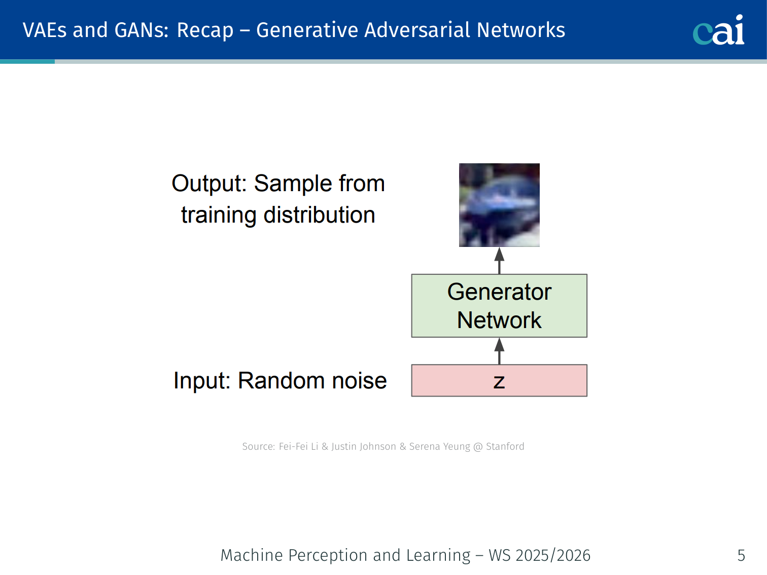
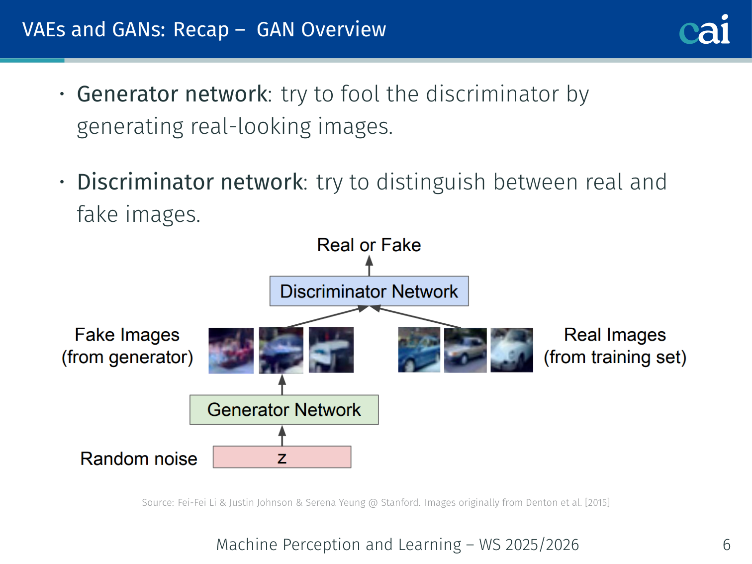
Here's how GANs work—the Generator and Discriminator constantly trying to outsmart each other.

The training in action as the Generator learns to turn random noise into something meaningful.

• Generator: try to fool the discriminator by generating real-looking images.
• Discriminator: try to distinguish between real and fake images.

	VAEs	GANs
Training	Relatively easier	Many tricks needed (mode collapse, adversarial objective)
Inference	Explicit encoder $q(z\mid x)$	Implicit generative model
Image quality	More blurry (reconstruction loss)	Sharper (discriminator loss)

---

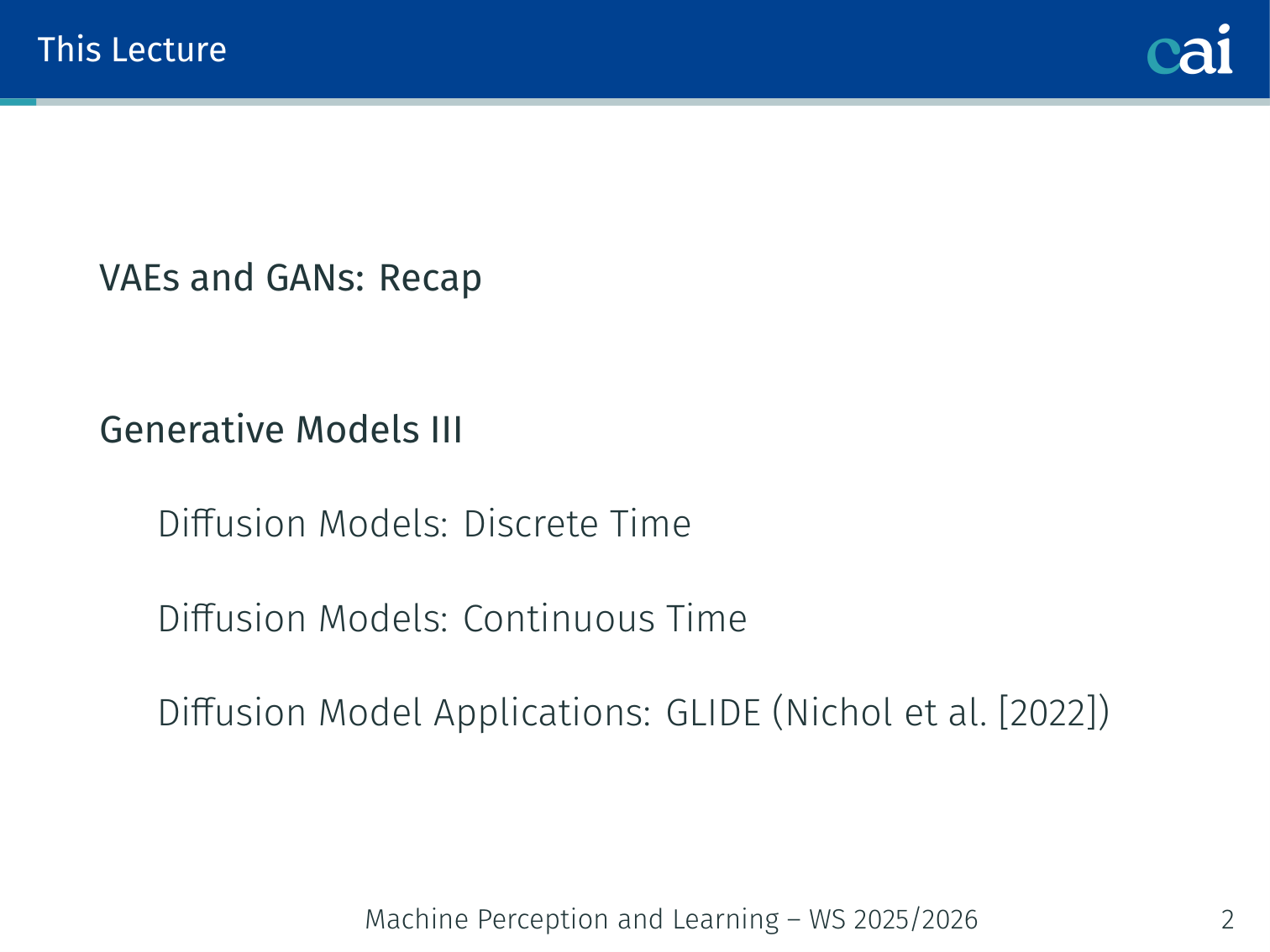
This Lecture — Generative Models III

---

Here's the plan for today: we'll cover everything from discrete diffusion to GLIDE.

1. Diffusion Models: Discrete Time
2. Diffusion Models: Continuous Time
3. Diffusion Model Application: GLIDE (Nichol et al., 2022)

Diffusion models have emerged as the most powerful generative models, outperforming GANs across image synthesis, super-resolution, text-to-image, video, 3D, and molecule generation.

---

Diffusion Models: Discrete Time

Basic Idea

Think of it as two halves: first we add noise, then we learn how to take it back out.

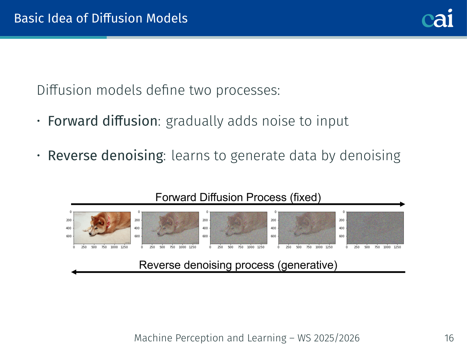
Diffusion models define two processes:

• Forward diffusion: gradually add noise to the input until only white noise remains.
• Reverse denoising: learn to generate data by iteratively denoising.

Forward:  x_0 (real) ──noise──► x_1 ──noise──► ... ──noise──► x_T (pure noise)
Reverse:  x_T (noise) ──denoise──► x_{T-1} ──► ... ──denoise──► x_0 (generated)

Example: Start with a photo of a dog. After T=1000 Gaussian noise steps, the image becomes indistinguishable from random Gaussian noise. A neural network trained to reverse this process can then go from noise back to a realistic dog photo.

---

Forward Diffusion Process

In the forward pass, we're just watching the image gradually dissolve into pure noise.

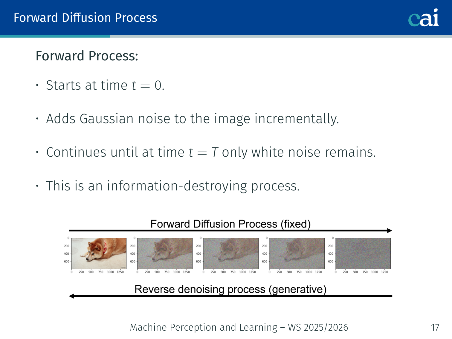
The forward process starts at $t=0$ and adds Gaussian noise incrementally via a Markov chain:

$q(x_t|x_{t-1})=\mathcal{N}\left(x_t;\sqrt{1-{\beta }_t}{x}_{t-1},{\beta }_t\mathbf{I}\right)$

• ${\beta }_t$ is the variance schedule — a hyperparameter controlling how much noise to add at step $t$.
• The process continues until $t=T$, where only white noise remains.
• This is an information-destroying Markov process.

The joint distribution over the entire forward trajectory:

$q(x_{1:T}|x_0)={\prod }_{t=1}^{T}q(x_t|x_{t-1})$

Noise Schedule Intuition

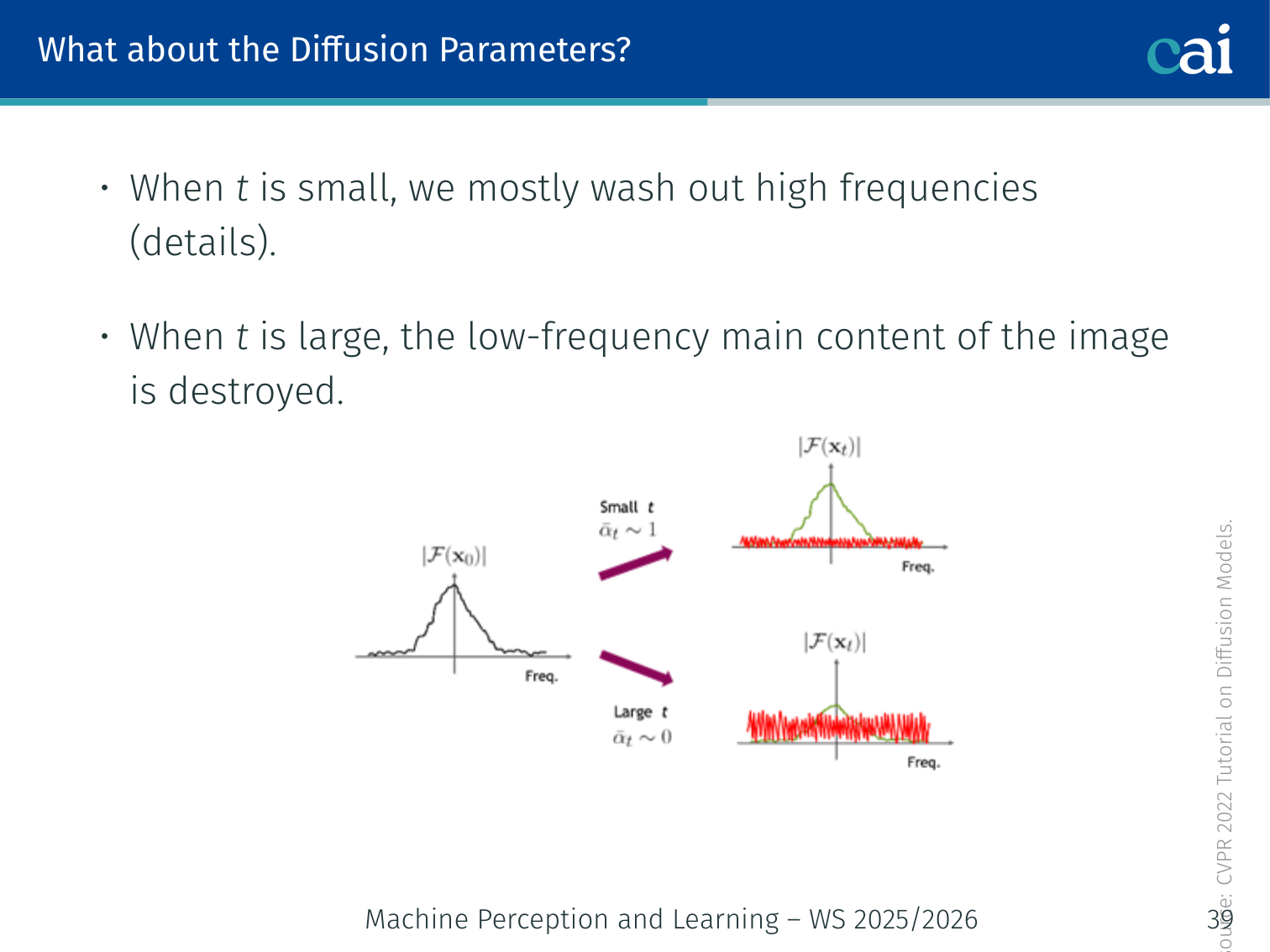
The noise schedule hits different frequencies at different stages of the process.

Timestep $t$	Effect
Small $t$	Mostly washes out high frequencies (fine details)
Large $t$	Destroys low-frequency content (main structure of the image)

Example: At $t=100$ a face image starts looking blurry (details lost). At $t=800$ only a rough blob is visible. At $t=1000$ it is pure noise.

---

Sampling from the Forward Distribution — Closed Form

The cool thing is this closed-form trick—we can jump straight to any noisy step we want.

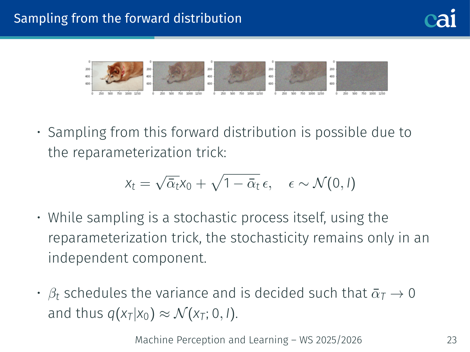
You do not need to simulate step-by-step. The reparameterization trick gives a closed form:

Define ${\alpha }_t=1-{\beta }_t$ and ${\bar{\alpha }}_t={\prod }_{i=1}^t{\alpha }_i$. Then:

$x_t=\sqrt{{\bar{\alpha }}_t}{x}_0+\sqrt{1-{\bar{\alpha }}_t}\epsilon ,\epsilon \sim \mathcal{N}(0,I)$

Or equivalently:

$q(x_t|x_0)=\mathcal{N}\left(x_t;\sqrt{{\bar{\alpha }}_t}{x}_0,(1-{\bar{\alpha }}_t)\mathbf{I}\right)$

As $t\to \infty$: ${\bar{\alpha }}_t\to 0$, so $q(x_T|x_0)\approx \mathcal{N}(0,I)$ — pure noise.

# Example: jump to any noisy step in one shot
def forward_sample(x0, t, alpha_bar):
    eps = torch.randn_like(x0)
    x_t = alpha_bar[t].sqrt() * x0 + (1 - alpha_bar[t]).sqrt() * eps
    return x_t, eps

Why this matters: Training doesn’t require running the full chain — sample a random $t$, perturb $x_0$ directly, and train on that.

💡 Intuition: Every Noisy Sample Is Just “Signal + Noise”

The closed-form equation

$x_t=\sqrt{{\bar{\alpha }}_t}{x}_0+\sqrt{1-{\bar{\alpha }}_t}\epsilon$

is worth memorizing conceptually, even if not symbol by symbol.

It says that any noisy sample $x_t$ is just:

• a shrunk copy of the original data $x_0$
• plus a scaled amount of Gaussian noise

Early in the chain, $\sqrt{{\bar{\alpha }}_t}$ is still large, so the image structure dominates. Late in the chain, $\sqrt{1-{\bar{\alpha }}_t}$ dominates, so almost everything is noise.

That is why denoising is possible at intermediate timesteps: the original signal has not fully disappeared yet.

---

How Does the Distribution Change?

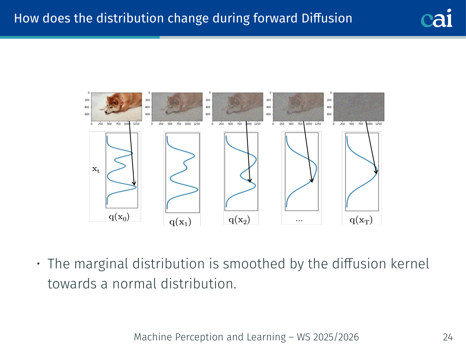
Watch how that complex data distribution eventually smooths out into a simple Gaussian.

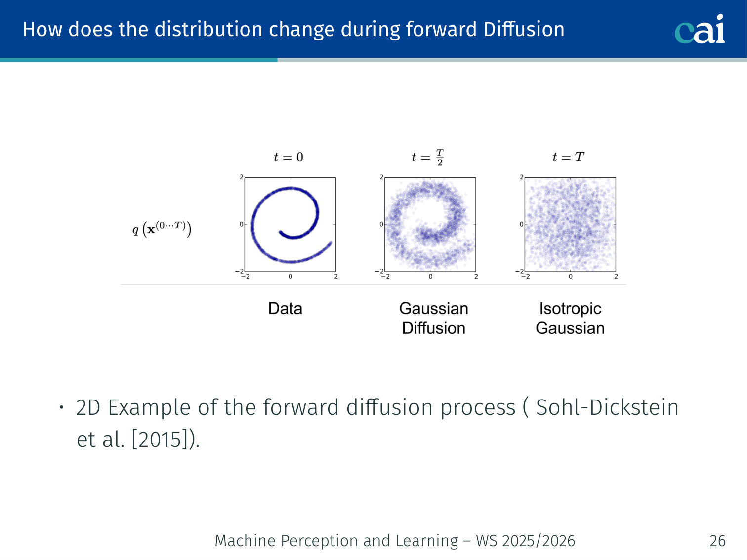
It's a mix of drift and diffusion, slowly turning that weird shape into a standard Gaussian blob.

During forward diffusion, the marginal distribution $q(x_t)$ is smoothed gradually toward $\mathcal{N}(0,I)$:

• Each step acts as a drift toward the mean + a diffusion (spread) term.
• In 2D (Sohl-Dickstein et al., 2015): a non-Gaussian data distribution smoothly becomes a Gaussian blob after many steps.

---

Generative Learning by Reversing the Diffusion Process

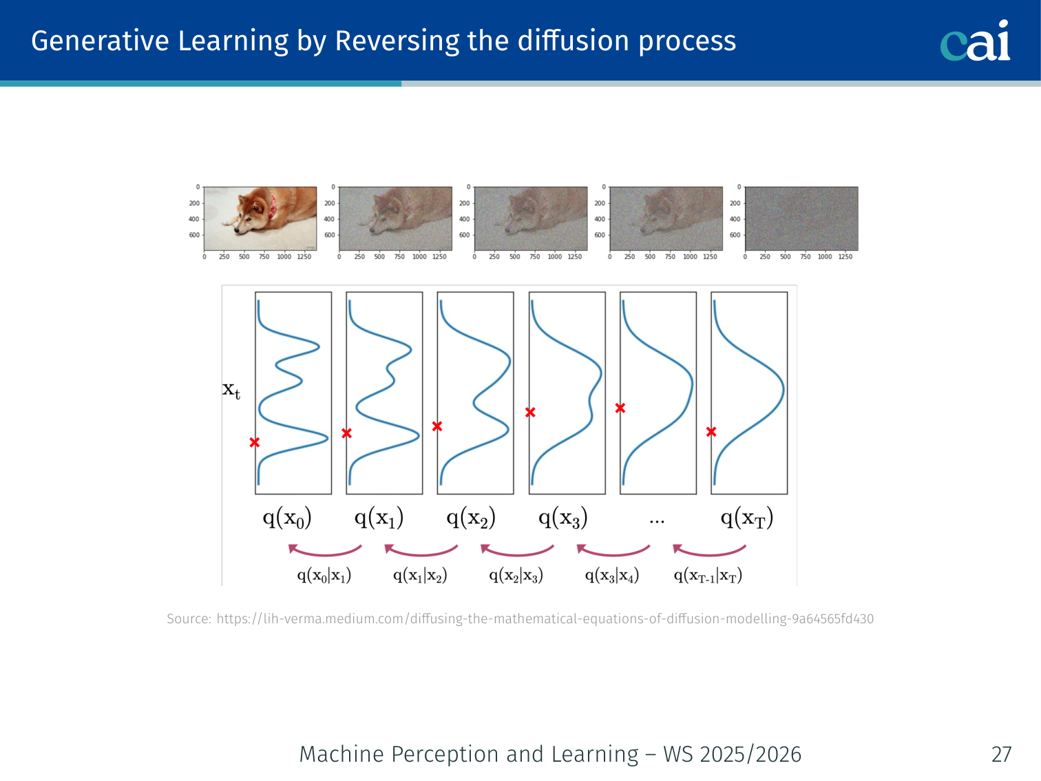
Now for the magic: learning to undo all that noise, one tiny step at a time.

To generate data, start from noise and reverse:

1. Sample $x_T\sim \mathcal{N}(0,I)$.
2. Iteratively sample $x_{t-1}\sim q(x_{t-1}|x_t)$ for $t=T,T-1,\dots ,1$.

Using Bayes’ rule:

$q(x_{t-1}|x_t)=\frac{q(x_t|x_{t-1})\cdot q(x_{t-1})}{q(x_t)}$

Problem: this requires access to the entire dataset (intractable). Also, if the timesteps are small enough, $q(x_{t-1}|x_t)$ is approximately Gaussian — so we can train a neural network to approximate it.

---

💡 Intuition: Denoising as “Climbing the Mountain of Data”

Diffusion models are like a search for where the data “lives”.

• The Forward Process: You start with a clear photo and walk away into a dense fog (adding noise) until you are completely lost.
• The Reverse Process (Learning): The model is like a compass. It learns to point in the direction where the photo used to be.

By predicting the noise, the model is actually telling you: “If you want to find the real image, move in this direction.” If you follow that compass 1000 times, you’ll walk out of the fog and end up at a high-quality photo.

---

🧠 Deep Dive: The Score Function

In continuous-time diffusion, we talk about the Score Function ${\nabla }_x\log p_t(x)$.

The Problem: We want to know how to move from a noisy image $x$ to a more realistic image. If we knew the probability distribution $p(x)$ of all real images, we would just move in the direction where the probability increases the fastest (the gradient).

The Solution: The denoiser network ${\epsilon }_{\theta }(x_t,t)$ is mathematically related to this score. When you train a network to predict noise, you are implicitly teaching it the Score Function. It learns the “shape” of the data distribution and can push random noise toward the peaks of that distribution — which are the realistic images.

---

Parametric Reverse Model

We use a parametric model $p_{\theta }$ to approximate the reverse process:

$p(x_T)=\mathcal{N}(x_T;0,I)$

$p_{\theta }(x_{t-1}|x_t)=\mathcal{N}\left(x_{t-1};{\mu }_{\theta }(x_t,t),{\sigma }_t^{2}I\right)$

The joint reverse distribution:

$p_{\theta }(x_{0:T})=p(x_T){\prod }_{t=1}^T{p}_{\theta }(x_{t-1}|x_t)$

---

Reverse Conditional Gaussian and Training Objective

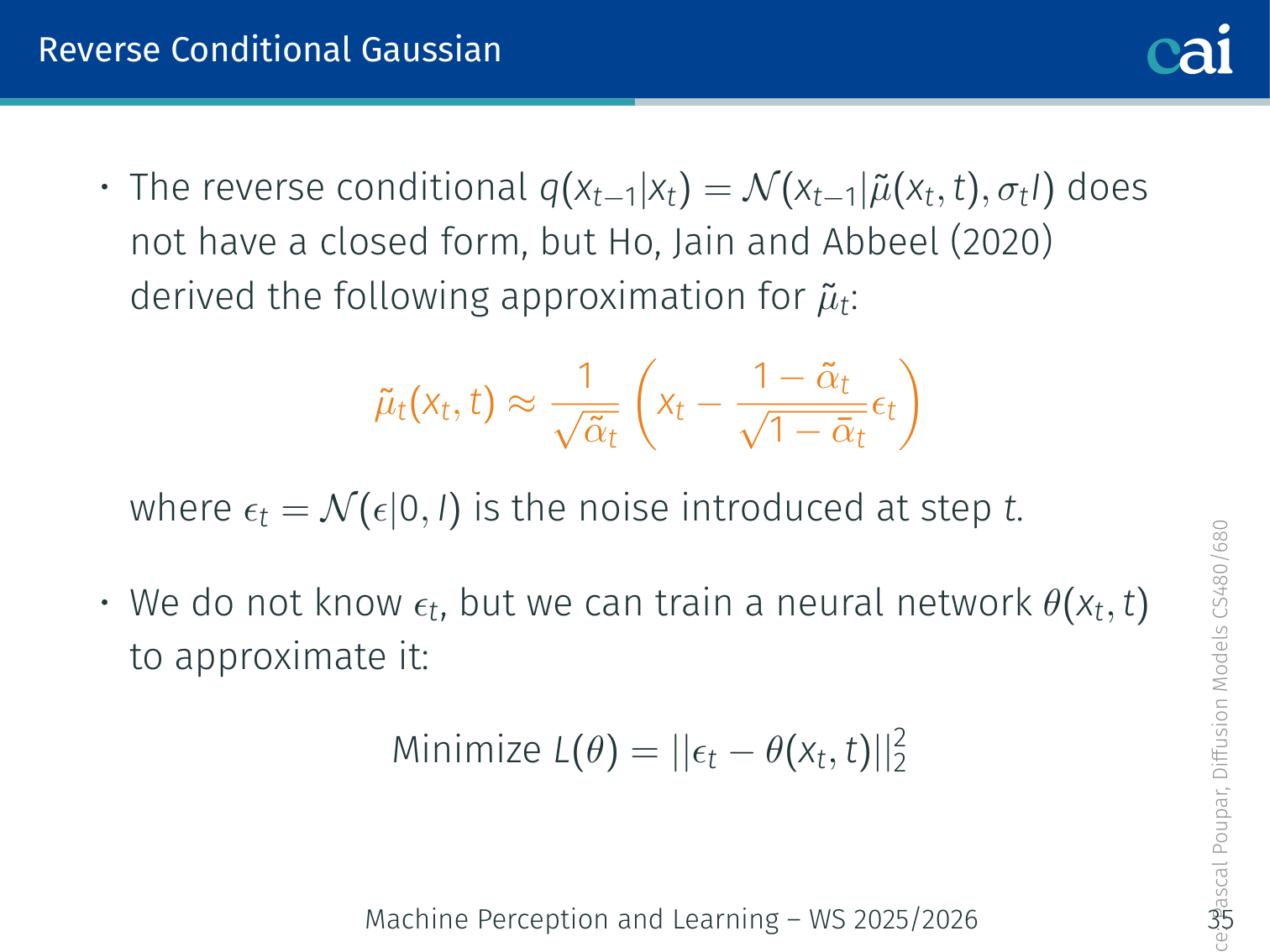
The goal for DDPM is simple—just make the predicted noise match the actual noise we added.

The reverse conditional $q(x_{t-1}|x_t)$ has no analytical closed form. However, Ho, Jain and Abbeel (2020) derived the following approximation for the reverse mean:

${\tilde{\mu }}_t(x_t,t)\approx \frac{1}{\sqrt{{\tilde{\alpha }}_t}}\left(x_t-\frac{1-{\tilde{\alpha }}_t}{\sqrt{1-{\bar{\alpha }}_t}}{\epsilon }_t\right)$

where ${\epsilon }_t\sim \mathcal{N}(0,I)$ is the noise introduced at step $t$.

Since we don’t know ${\epsilon }_t$ at inference time, we train a neural network $\theta (x_t,t)$ to predict it:

$\mathcal{L}(\theta )=\Vert {\epsilon }_t-\theta (x_t,t){\Vert }_2^2$

This is a simple MSE loss — predict the noise added, nothing more.

# DDPM training loop (Ho et al., 2020)
for x0 in dataloader:
    t   = torch.randint(0, T, (x0.shape[0],))   # random timestep
    eps = torch.randn_like(x0)                    # true noise
 
    # Closed-form noisy sample
    x_t = sqrt_alpha_bar[t] * x0 + sqrt_one_minus_alpha_bar[t] * eps
 
    # Predict the noise with the U-Net
    eps_pred = unet(x_t, t)
 
    # Minimize MSE
    loss = F.mse_loss(eps_pred, eps)
    loss.backward()
    optimizer.step(); optimizer.zero_grad()

Intuition: The model learns “what noise was added to get this blurry image?” By subtracting the predicted noise, it recovers a cleaner version — one step of denoising.

🧠 Deep Dive: Why Predict the Noise Instead of the Clean Image?

There are several equivalent parameterizations in diffusion models: predict $x_0$, predict the reverse-process mean, or predict the noise $\epsilon$.

The original DDPM paper shows why $\epsilon$-prediction became the standard teaching version:

• it simplifies the variational objective into a clean denoising loss
• it connects directly to denoising score matching
• empirically, Ho et al. report that predicting $x_0$ gave worse sample quality early in their experiments

So “predict the noise” is not just a coding convenience. It is the parameterization that made the method both conceptually cleaner and empirically stronger.

---

Training Procedure — U-Net Architecture

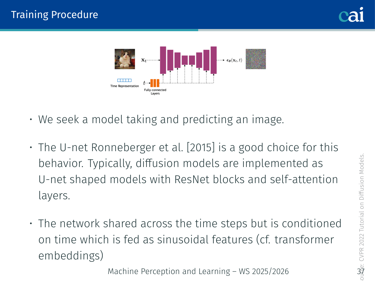
We're using a U-Net here, complete with skip connections and time-step embeddings to handle the denoising.

The denoiser network $\theta (x_t,t)$ takes a noisy image and predicts the added noise.

The U-Net (Ronneberger et al., 2015) is a natural choice:

Input: noisy image (H × W × C)
          │
   ┌──────┴──────┐
   │  Encoder    │  Conv + ResBlocks + Self-Attention
   │  (downsample)│
   └──────┬──────┘
          │
   Bottleneck (self-attention)
          │
   ┌──────┴──────┐
   │  Decoder    │  Conv + ResBlocks + Self-Attention
   │  (upsample) │← skip connections from encoder
   └──────┬──────┘
          │
Output: predicted noise (H × W × C)

• The same network is shared across all timesteps.
• Time $t$ is encoded as sinusoidal features (like transformer positional encodings) and injected into every ResBlock.

Example: At $t=500$, the U-Net receives a half-noisy cat image and predicts the noise component. At $t=10$, it receives an almost-clean image and predicts a small residual noise.

---

Diffusion Hyperparameters — The Noise Schedule

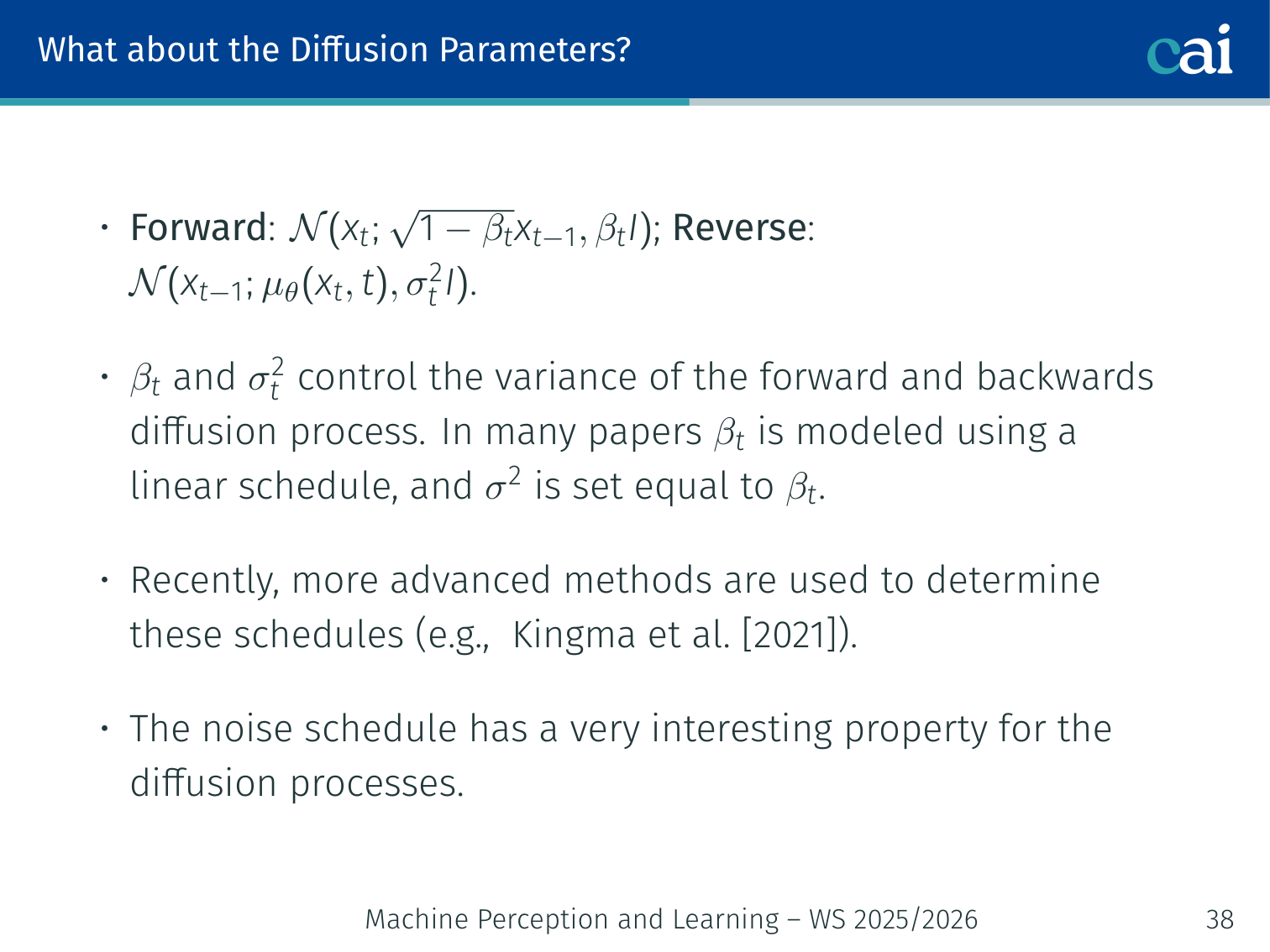
Adjusting these hyperparameters really changes how the noise builds up over time.

Forward: $\mathcal{N}(x_t;\sqrt{1-{\beta }_t}{x}_{t-1},{\beta }_{t}I)$ — Reverse: $\mathcal{N}(x_{t-1};{\mu }_{\theta }(x_t,t),{\sigma }_t^{2}I)$

• ${\beta }_t$ and ${\sigma }_t^2$ control the variance of the forward and backward processes.
• In many papers ${\beta }_t$ follows a linear schedule and ${\sigma }_t^2={\beta }_t$.
• More advanced schedules exist (e.g., Kingma et al., 2021 — cosine schedule).

# Linear beta schedule example
T    = 1000
beta = torch.linspace(1e-4, 0.02, T)          # β_1 ... β_T
alpha     = 1 - beta
alpha_bar = torch.cumprod(alpha, dim=0)        # ᾱ_t

Why the schedule matters: too aggressive ${\beta }_t$ destroys signal too quickly; too gentle leaves structure at $t=T$, breaking the Gaussian assumption.

---

Connection to VAEs

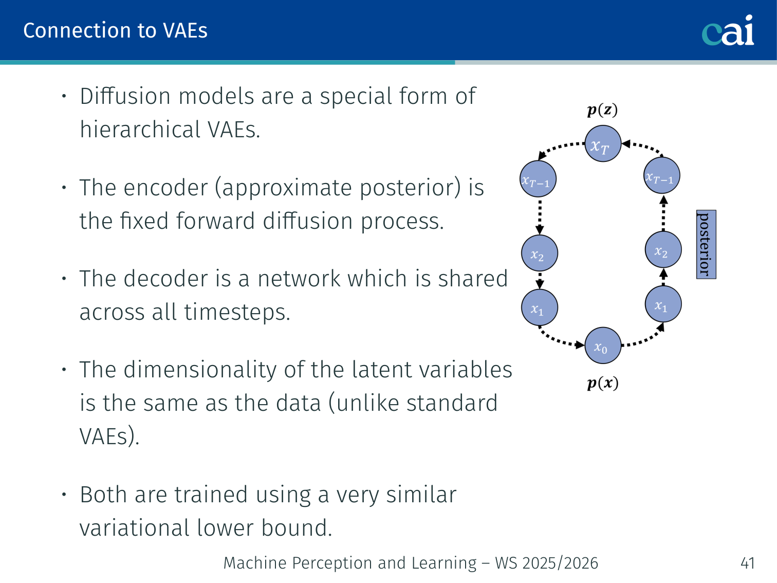
If you look closely, diffusion models and hierarchical VAEs actually share a lot of the same DNA.

Diffusion models are a special form of hierarchical VAEs:

	Standard VAE	Diffusion Model
Encoder (posterior)	Learned $q_{\varphi }(z\mid x)$	Fixed forward process $q(x_{1:T}\mid x_0)$
Decoder	Learned $p_{\theta }(x\mid z)$	Shared network $p_{\theta }(x_{t-1}\mid x_t)$ across all $t$
Latent dimensionality	Smaller than input	Same as input
Training objective	ELBO	Very similar variational lower bound

💡 Intuition: Why People Say Diffusion Is “Like a VAE”

The comparison is useful because both models can be read as latent-variable generative models trained with a variational objective.

The big difference is what counts as the latent code:

• in a standard VAE, one compact latent $z$ tries to summarize the whole example
• in diffusion, the latent variables are the entire noisy trajectory $x_1,\dots ,x_T$

So diffusion spreads the generative problem across many easy denoising steps instead of asking one bottleneck vector to carry everything at once. That is one reason it tends to generate higher-quality samples than a plain VAE.

---

Diffusion Models: Continuous Time

SDE Formulation (Song et al., 2021)

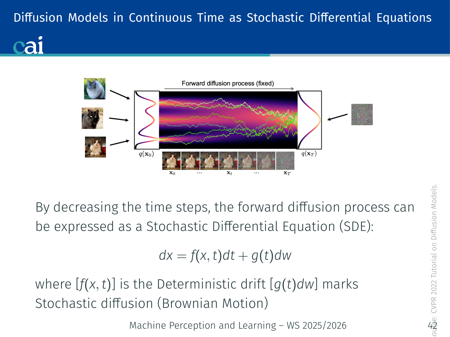
Let's look at this from a continuous perspective using Stochastic Differential Equations.

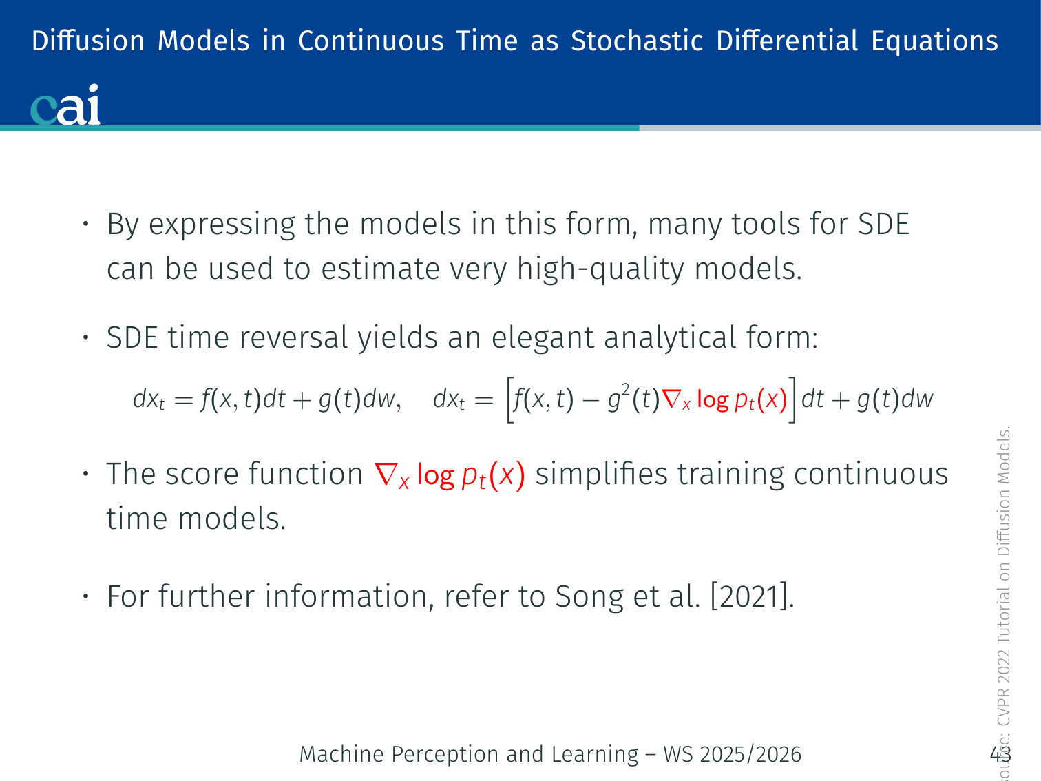
As the number of timesteps $T\to \infty$, the discrete Markov chain becomes a Stochastic Differential Equation (SDE):

$dx=f(x,t)dt+g(t)dw$

• $f(x,t)$: deterministic drift term
• $g(t)dw$: stochastic diffusion term (Brownian motion)

Time Reversal

Reversing the time in these SDEs really comes down to mastering the score function.

SDE time reversal yields an elegant analytical form for the reverse (generative) SDE:

$d{x}_t=\left[f(x,t)-g^2(t){\nabla }_x\log p_t(x)\right]dt+g(t)dw$

The term ${\nabla }_x\log p_t(x)$ is the score function — the gradient of the log data density at noise level $t$. This is precisely what the denoiser network learns to estimate.

Why this matters: Expressing diffusion as an SDE opens access to the full toolkit of stochastic calculus — ODE solvers, higher-order integrators, and theoretical convergence guarantees. It unifies DDPM, DDIM (which is a probability-flow ODE), and score-based models under one framework.

---

Discussion: Advantages and Disadvantages

Advantages

• High diversity: covers the data distribution well, unlike mode-collapsing GANs.
• High quality: samples are comparable to or better than GANs.
• Flexible conditioning: easily conditioned on images, text, or class labels.

Disadvantages

• Slow generation: requires many forward passes through the network ($T=1000$ steps by default).
• Less meaningful latents: latent variables have the same dimensionality as the data — harder to interpret or manipulate.

---

The Generative Trilemma

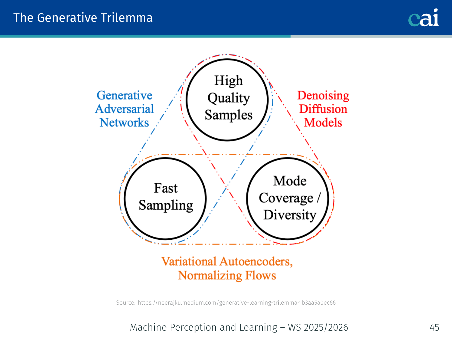
The classic generative trilemma: you're always balancing quality, sampling speed, and diversity.

Most generative models can excel at only two of three desirable properties:

             HIGH QUALITY
                  △
                 /|\
                / | \
               /  |  \
              /   |   \
FAST SAMPLING ──────────── HIGH DIVERSITY
                             (mode coverage)

Model	Quality	Diversity	Speed
GANs	✅ High	❌ Mode collapse	✅ 1 pass
VAEs	⚠️ Blurry	✅ Good	✅ 1 pass
Diffusion (DDPM)	✅ High	✅ Full distribution	❌ 1000 steps

Diffusion often offers strong quality and coverage, but usually sacrifices speed — motivating DDIM, consistency models, and flow matching.

DDIM — Fast Sampling

DDPM sampling is high quality but slow: at inference time it often requires $T=1000$ denoising steps. This is one of the main practical bottlenecks of diffusion models.

DDIM (Denoising Diffusion Implicit Models) addresses this by introducing a non-Markovian forward process that keeps the same training objective but allows much faster and even deterministic sampling (Song et al., 2020).

Key Idea: Skip Timesteps

Instead of following every single reverse step

$$T\to T-1\to T-2\to \cdots \to 0$$

DDIM chooses a shorter subsequence of timesteps

$$\tau =\{t_1,t_2,\dots ,t_S\},S\ll T$$

and jumps directly along this shorter trajectory.

So at inference we can use, for example, 50 steps instead of 1000.

DDIM Update Rule

As in DDPM, first estimate the clean sample:

$${\hat{x}}_0=\frac{x_t-\sqrt{1-{\bar{\alpha }}_t}{\epsilon }_{\theta }(x_t,t)}{\sqrt{{\bar{\alpha }}_t}}$$

Then the general DDIM update from $t_i$ to $t_{i-1}$ is

$$x_{t_{i-1}}=\sqrt{{\bar{\alpha }}_{t_{i-1}}}{\hat{x}}_0+\sqrt{1-{\bar{\alpha }}_{t_{i-1}}-{\sigma }_{t_i}^2}{\epsilon }_{\theta }(x_{t_i},t_i)+{\sigma }_{t_i}z,z\sim \mathcal{N}(0,I)$$

For deterministic DDIM sampling, set ${\sigma }_{t_i}=0$:

$$x_{t_{i-1}}=\sqrt{{\bar{\alpha }}_{t_{i-1}}}{\hat{x}}_0+\sqrt{1-{\bar{\alpha }}_{t_{i-1}}}{\epsilon }_{\theta }(x_{t_i},t_i)$$

So DDIM can be viewed as tracing a deterministic path through latent space when desired.

💡 Intuition: Why DDIM Can Use the Same Training Objective

The clever part of DDIM is that it changes the sampling dynamics without requiring a new model to be trained from scratch.

The DDIM paper’s core claim is exactly this: construct a non-Markovian process that preserves the same training objective as DDPM, but gives you a faster reverse process.

So the model still learns the same kind of denoising prediction. What changes is the path you choose at inference time.

Example: Instead of denoising along 999 -> 998 -> 997 -> ... -> 0, DDIM may use a much shorter path such as 999 -> 979 -> 959 -> ... -> 19 -> 0.

Why It Matters

In practice, DDIM can retain useful sample quality with far fewer steps than DDPM, often making diffusion models much more usable at inference time.

Code: Skipping Timesteps with a Stride

# Example: deterministic DDIM with a strided timestep schedule
S = 50
stride = T // S
timesteps = list(range(T - 1, -1, -stride))
 
x = torch.randn(1, 3, 64, 64)
 
for i, t in enumerate(timesteps[:-1]):
    t_prev = timesteps[i + 1]
 
    eps = model(x, torch.tensor([t]))
    x0_hat = (x - (1 - alpha_bar[t]).sqrt() * eps) / alpha_bar[t].sqrt()
 
    # DDIM with eta = 0 -> deterministic update
    x = alpha_bar[t_prev].sqrt() * x0_hat + (1 - alpha_bar[t_prev]).sqrt() * eps

The essential trick is simple: define a shorter timestep schedule and denoise only on that schedule.

---

Latent Diffusion Models (Rombach et al., 2022)

Motivation — The Scaling Problem

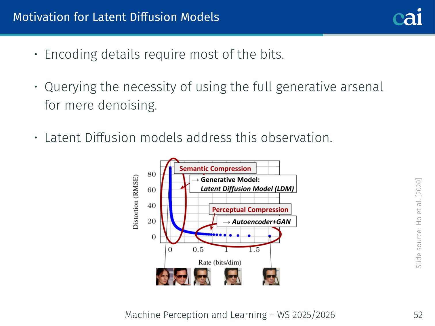
Working directly in high-res pixel space is a massive computational headache.

Diffusion models do not scale well with image resolution. A 512×512×3 pixel image has ~786K dimensions, making direct pixel-space diffusion computationally expensive.

Observation (Ho et al., 2020): most “bits” in an image encode fine-grained perceptual detail, not semantic content. Running the full generative process in pixel space wastes computation on imperceptible differences.

The lecture motivates this with a rate-distortion view: fine-grained perceptual details consume most of the bit budget, while the more semantically meaningful structure can often be modeled in a much smaller latent space. Latent diffusion therefore splits the problem into:

• Perceptual compression: let an autoencoder preserve visually important detail
• Semantic compression: let diffusion model the higher-level structure in latent space

Two common strategies:

1. Downsample → process at smaller scale → upsample.
2. Translate to latent space → run diffusion in latent space → decode back.

💡 Intuition: Latent Diffusion Is “Compress First, Generate Second”

Latent diffusion works because not every pixel-level detail deserves equal generative effort.

The autoencoder handles the low-level perceptual bookkeeping:

• textures
• local image detail
• reconstruction back to pixel space

Then the diffusion model can spend its capacity on the harder, more semantic question:

• what objects are present?
• how are they arranged?
• what should the image mean overall?

So latent diffusion is really a division of labor:

• autoencoder for efficient perceptual compression
• diffusion model for semantic generation in a smaller, cheaper space

Architecture

$x_0\stackrel{\text{VAE Encoder}}{\to }{z}_0\stackrel{\text{Add noise}}{\to }{z}_T\stackrel{\text{Denoiser }{\epsilon }_{\theta }(z_t,t,c)}{\to }{\hat{z}}_0\stackrel{\text{VAE Decoder}}{\to }{\hat{x}}_0$

• The VAE encoder maps input data to a compressed embedding (e.g., 64×64×4 for a 512×512 image — 96× smaller).
• Denoising diffusion is applied in the latent space.
• A patch-based adversarial discriminator is added on top of the reconstruction loss for perceptual compression.
• The VAE decoder reconstructs the final image from the denoised latent.

Text Prompt c ─────────────────────────────── (cross-attention)
                                                      │
x_0 →[VAE Enc]→ z_0 →[Noise]→ z_T →[U-Net]→ ẑ_0 →[VAE Dec]→ x̂_0

Two-Stage Training

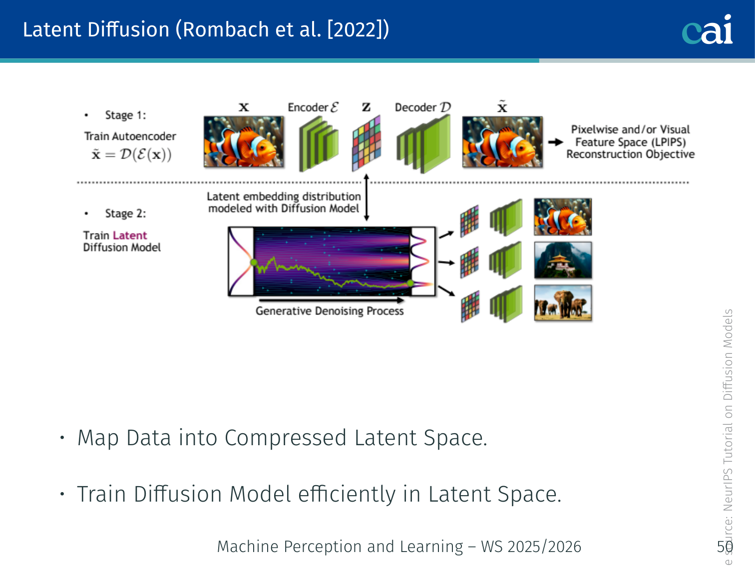
The trick with Latent Diffusion is to compress the image first, then do all the heavy lifting in that smaller space.

Latent diffusion is trained in two stages:

1. Train the autoencoder first so that $x\to z\to \hat{x}$ preserves perceptually relevant content
2. Train the diffusion model on latents $z$ instead of pixels

🧠 Deep Dive: Why Cross-Attention Became So Important in LDMs

The latent diffusion paper highlights another major idea beyond compression: cross-attention turns diffusion into a flexible conditional generator.

Why is cross-attention such a good fit for text-to-image?

• the image latents keep their spatial structure
• the text tokens stay as a sequence
• cross-attention lets each spatial location query whichever words matter most

That means the model does not have to squash the whole prompt into one vector. Different parts of the image can attend to different words such as “red”, “apple”, “wooden”, or “table” at the same time.

This is a big part of why latent diffusion became the foundation for systems like Stable Diffusion.

In the lecture slides, the first stage is not just plain reconstruction: a patch-based adversarial discriminator is added on top of the reconstruction / perceptual objective so the latent space keeps visually important details while staying compressed.

Advantages of Latent Diffusion

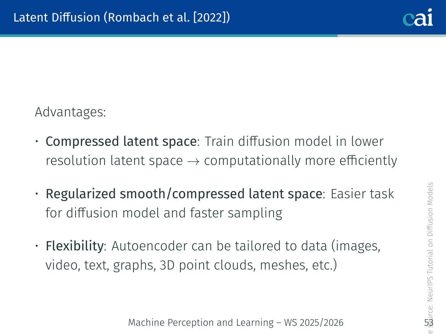
Latent Diffusion gives us the best of both worlds: it's efficient and handles semantics way better.

Benefit	Explanation
Compressed latent space	Train diffusion in low-resolution latent → computationally efficient
Regularized/smooth space	Easier denoising task, faster sampling than pixel-space
Flexibility	The autoencoder can be adapted to images, video, text, graphs, 3D point clouds, meshes, etc.

Example — Stable Diffusion: A 512×512 image is encoded into a 64×64×4 latent. All 1000 denoising steps happen in this small latent space, then a single decoder pass produces the final image. This enables high-quality image generation on a consumer GPU.

---

Application: GLIDE (Nichol et al., 2022)

Overview

GLIDE lets us both generate new images and edit existing ones just by typing a prompt.

GLIDE = Guided Language-to-Image Diffusion

• 3.5 billion parameter text-conditional diffusion model.
• Supports two guidance strategies: CLIP guidance and classifier-free guidance.

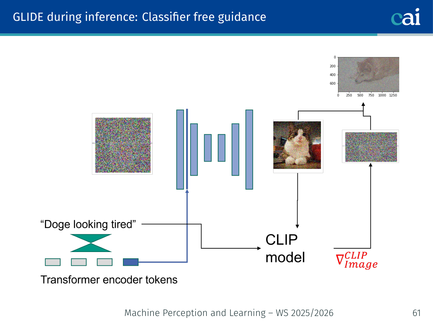
CLIP Guidance (Radford et al., 2021)

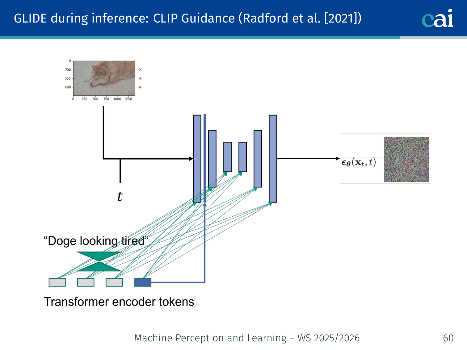
We can use CLIP to steer the diffusion process by checking how well the image matches our text.

CLIP is a large model that takes an image $x$ and a text $c$ and outputs a similarity score.

• The CLIP gradient ${\nabla }_x{\mathcal{L}}_{\text{CLIP}}(f(x_t),g(c))$ points in the direction of images that better match the text.
• This gradient steers the diffusion process during inference.

The combined objective:

${\nabla }_x\mathcal{L}={\nabla }_x{\mathcal{L}}_{\text{data}}(x_t,c)+s\cdot {\nabla }_x{\mathcal{L}}_{\text{CLIP}}(f(x_t),g(c))$

• $s$ is the guidance strength.
• $f$ = image encoder, $g$ = text encoder.

Example: When generating “a red apple on a wooden table”, the CLIP gradient nudges each denoising step toward images whose visual features are more similar to that text description.

🧠 Deep Dive: Classifier-Free Guidance (CFG)

If you’ve ever used a tool like Stable Diffusion and adjusted the “Guidance Scale” or “CFG Scale,” this is what’s happening under the hood.

The Goal: We want the model to follow our text prompt $c$ as closely as possible.

The Solution: During training, we randomly “drop out” the text prompt (e.g., 10% of the time, we show the model an empty string $\varnothing$). This teaches the model two things:

1. $p(x_t|c)$: How to generate an image based on a prompt.
2. $p(x_t)$: How to generate any random image.

At Inference: We calculate the noise for both the prompt and the empty prompt, then amplify the gap between them.

The original classifier-free guidance paper writes this as:

$\tilde{\epsilon }=(1+w){\epsilon }_{\text{cond}}-w{\epsilon }_{\text{uncond}}$

Many practical codebases write an equivalent form using a guidance scale $s=w+1$:

$\tilde{\epsilon }={\epsilon }_{\text{uncond}}+s\cdot ({\epsilon }_{\text{cond}}-{\epsilon }_{\text{uncond}})$

• Low guidance: more diverse, but weaker prompt adherence.
• High guidance: stronger prompt adherence, but lower diversity and possible oversaturation artifacts.

---

GLIDE Training

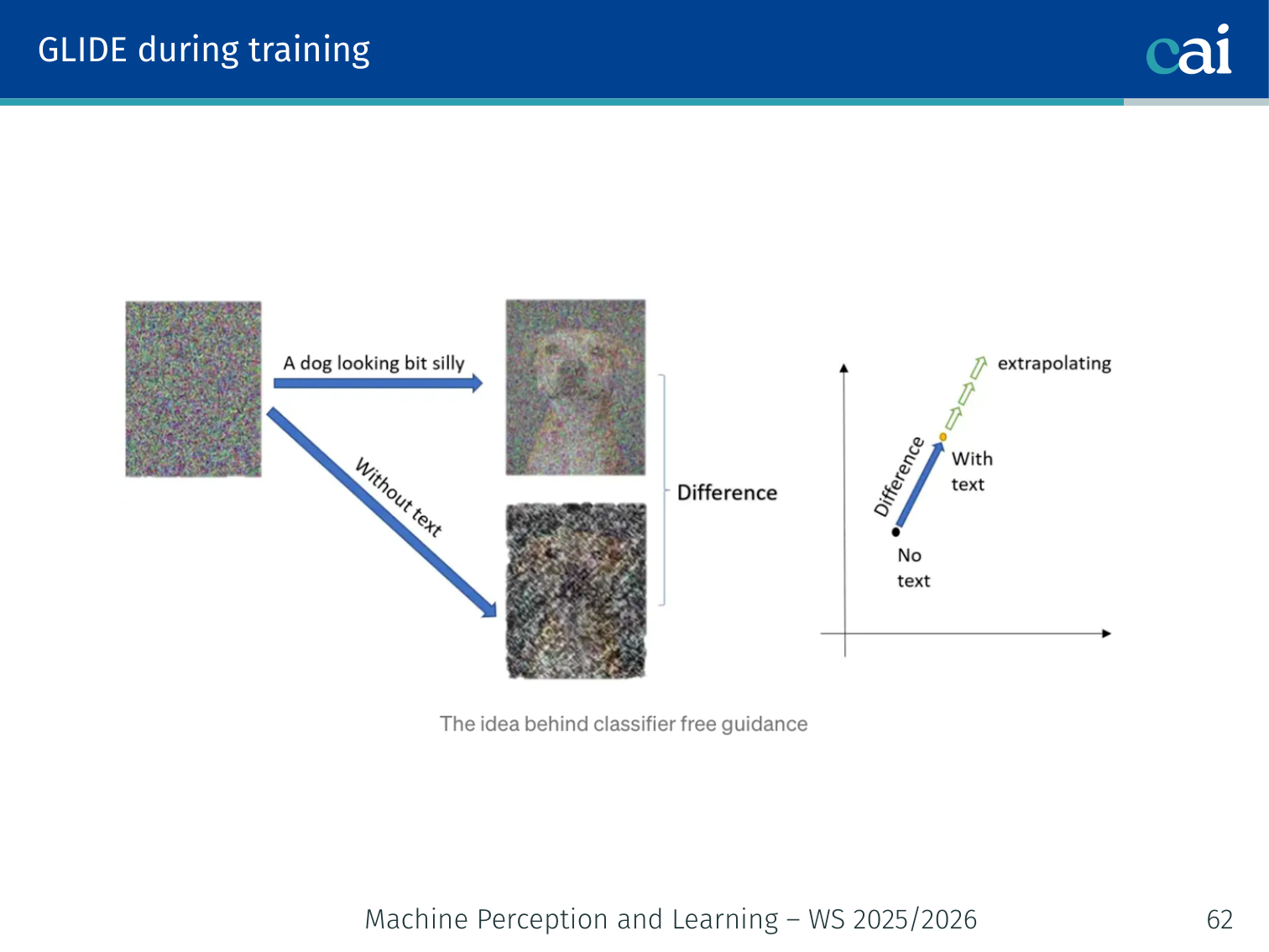
Training GLIDE involves teaching it to denoise both with and without the text prompt.

The lecture’s training slide clarifies how classifier-free guidance is enabled: during training, GLIDE is randomly asked to denoise with text conditioning and without text conditioning. That means the same network learns both:

• a generic unconditional denoiser
• a prompt-conditioned denoiser

The difference between these two predictions becomes the direction that is later amplified at inference time.

Classifier-Free Guidance (Ho & Salimans, 2022)

Classifier-free guidance is basically just sliding between the conditional and unconditional predictions.

Problem: Conditional generation doesn’t always follow the text prompt closely enough.

Solution: Train one model for both conditional and unconditional generation. Randomly drop the text condition during training (replace $c$ with $\varnothing$). At inference, extrapolate away from the unconditional direction:

$\hat{\epsilon }={\epsilon }_{\theta }(x_t,t,\varnothing )+w\cdot \left[{\epsilon }_{\theta }(x_t,t,c)-{\epsilon }_{\theta }(x_t,t,\varnothing )\right]$

• In many implementations, $w$ is the guidance scale, where $w=1$ recovers the ordinary conditional prediction and larger values add extrapolative guidance.
• In the original Ho-Salimans paper, the coefficient is parameterized slightly differently; the paper’s $w$ corresponds to guidance_scale - 1 in the common implementation form above.
• Larger guidance improves prompt adherence but usually reduces diversity.

The lecture explicitly notes that the best GLIDE results are obtained with classifier-free guidance, rather than the external CLIP-guided variant.

# Classifier-free guidance at inference
eps_uncond = model(x_t, t, cond=None)          # unconditional prediction
eps_cond   = model(x_t, t, cond=text_emb)      # conditional prediction
eps_guided = eps_uncond + w * (eps_cond - eps_uncond)  # guided prediction

Example:

• $w=1.0$ → “a painting of a sunset” produces a vague, diverse sunset.
• $w=7.5$ → the prompt is followed closely, boats and horizon are clearly visible.
• $w=15$ → very strong adherence but may produce over-saturated artifacts.

GLIDE Editing Results

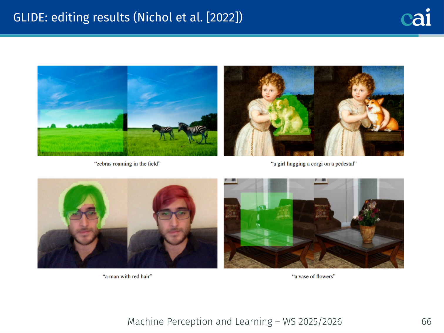
Here are some cool examples of GLIDE doing its thing with text-guided edits and inpainting.

GLIDE is not only a text-to-image generator from scratch; the lecture’s editing slide shows it can perform text-guided local edits while preserving the rest of the image. The examples include:

• inserting zebras into an empty field
• editing a painting into “a girl hugging a corgi on a pedestal”
• changing a person’s hair to red
• replacing a masked table region with a vase of flowers

This is the same general diffusion machinery applied in an editing / inpainting-style setting: keep most of the scene fixed, but regenerate the masked region so it becomes consistent with the prompt.

---

Are We Done? — Open Challenges

A quick wrap-up of where we're still struggling with diffusion research.

• Research on key diffusion model elements is ongoing.
• Accelerating the diffusion process remains a central challenge.
• Many small update steps are needed to keep the reverse process invertible.

---

Summary

Concept	Key Detail
Forward process	Markov chain: add Gaussian noise step-by-step until $x_T\approx \mathcal{N}(0,I)$
Closed-form noisy sample	$x_t=\sqrt{{\bar{\alpha }}_t}{x}_0+\sqrt{1-{\bar{\alpha }}_t}\epsilon$ — jump to any $t$ directly
Reverse process	Parametric Gaussian: $p_{\theta }(x_{t-1}\mid x_t)=\mathcal{N}({\mu }_{\theta }(x_t,t),{\sigma }_t^{2}I)$
Training loss	$\mathcal{L}(\theta )=\Vert \epsilon -\theta (x_t,t){\Vert }_2^2$ — simple noise prediction MSE
Network	U-Net with ResBlocks + self-attention; time $t$ injected via sinusoidal embeddings
Noise schedule	${\beta }_t$ (linear or cosine) controls how fast structure is destroyed
Connection to VAEs	Diffusion = hierarchical VAE with fixed encoder, shared decoder
Continuous time	SDE: $dx=f(x,t)dt+g(t)dw$; reverse uses score ${\nabla }_x\log p_t(x)$
Generative trilemma	Diffusion: high quality + high diversity, but slow
Latent diffusion	Two-stage setup: perceptually compress with an autoencoder, then diffuse in VAE latent space
CLIP guidance	Gradient of CLIP similarity steers denoising toward text description
Classifier-free guidance	Train with and without text, then amplify $({\epsilon }_{\text{cond}}-{\epsilon }_{\text{uncond}})$ by scale $w$
GLIDE editing	Text-guided masked edits preserve global scene context while changing selected regions

PyTorch Implementation: Denoising Diffusion Probabilistic Models (DDPM)

DDPM works by gradually adding noise to data (forward) and then learning to reverse this process (backward) using a neural network.

import torch
import torch.nn as nn
 
class DDPM(nn.Module):
    def __init__(self, denoiser_net, T=1000):
        super().__init__()
        self.denoiser = denoiser_net # Usually a U-Net architecture
        self.T = T
 
        # 1. Setup the Linear Noise Schedule
        # betas: amount of noise added at each step t
        self.betas = torch.linspace(1e-4, 0.02, T)
        self.alphas = 1. - self.betas
        # alphas_cumprod (alpha_bar): the product of all alphas up to step t
        # This allows jumping from x_0 to x_t in one step
        self.alphas_cumprod = torch.cumprod(self.alphas, axis=0)
 
    def forward_diffusion(self, x_0, t):
        """
        Forward Process: Add noise to the clean data x_0 at timestep t.
        Mathematically: x_t = sqrt(alpha_bar) * x_0 + sqrt(1 - alpha_bar) * noise
        """
        noise = torch.randn_like(x_0)
        # Reshape alpha_bar to match image dimensions (Batch, 1, 1, 1)
        alpha_bar = self.alphas_cumprod[t].view(-1, 1, 1, 1)
 
        # Linearly combine the clean image and random noise
        x_t = torch.sqrt(alpha_bar) * x_0 + torch.sqrt(1 - alpha_bar) * noise
        return x_t, noise
 
    def denoise(self, x_t, t):
        """
        Backward Process: Use the trained network to predict the noise
        that was added to x_t at timestep t.
        """
        return self.denoiser(x_t, t)

Key Diffusion Concepts:

• The “One-Shot” Forward Pass: Thanks to the alpha_bar trick, we don’t have to simulate 1000 steps of noise to train the model. We can pick any t and calculate x_t directly.
• Predicting the Noise: Interestingly, it is easier for the network to predict the noise $ϵ$ than to predict the clean image $x_0$ directly.
• U-Net with Time Embedding: Since the network is shared across all 1000 steps, it needs to know which step it’s working on. Timestep t is usually converted into a vector and added to the network’s features.

---

References

• Song, Meng, Ermon (2020) — Denoising diffusion implicit models. arXiv:2010.02502.

Applied Exam Focus

• Forward Process: Gradually adds Gaussian noise to an image until it is pure noise. This is fixed and has no learnable parameters.
• Reverse Process: A U-Net is trained to predict the noise added at each step, effectively “undoing” the corruption to recover the image.
• Sampling: Unlike VAEs or GANs (one-step), Diffusion requires iterative refinement, making it high-quality but slower to generate.

---

Previous: L11 — RL | Back to MPL Index | Next: (y-13) XAI | (y) Return to Notes | (y) Return to Home