L13 — Explainable AI (XAI)

Previous: L12 — Diffusion | Back to MPL Index

Mental Model First

• XAI is not one single thing: some methods explain this prediction, some summarize global behavior, and some propose what would need to change.
• An explanation can feel convincing and still be misleading, so explanation quality has to be evaluated, not assumed.
• In practice, XAI is most useful for debugging, auditing, trust calibration, and surfacing spurious shortcuts.
• If one question guides this lecture, let it be: what kind of explanation do I actually need for the decision I am trying to understand?

Motivation

This is why we need XAI—especially when the model is making high-stakes decisions.

Model understanding is critical in domains involving high-stakes decisions. Without it, models remain opaque black boxes that can fail silently and destructively.

Why model understanding matters:

Reason	Description
Debugging	Diagnose why a model misbehaves
Bias detection	Identify unfair patterns across demographic groups
Recourse	Tell individuals what they could change to get a different outcome
Trust calibration	Know when (and when not) to trust a prediction
Deployment vetting	Assess whether a model is safe for real-world use

Motivating example — Wolf vs. Husky classifier: A canonical XAI cautionary tale is a classifier that appears to distinguish wolves from huskies, but explanation methods reveal that it is mostly reacting to snow in the background. The point of the example is that a model can be right for the wrong reason, and XAI can expose that before deployment.

---

Achieving Model Understanding

Two approaches exist:

Approach 1 — Inherently Interpretable Models

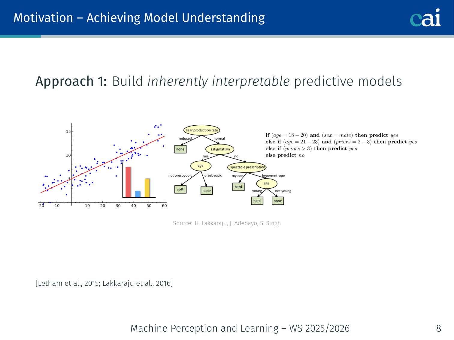
Some models, like decision trees, are actually pretty easy to understand right out of the box.

Build a model that is interpretable by design: decision trees, rule lists, linear classifiers, scoring systems [Letham et al., 2015; Lakkaraju et al., 2016].

• If Education ≤ High School → Salary ≤ 50k (a rule list)
• Transparent, auditable, but may sacrifice predictive power

Approach 2 — Post-hoc Explanations

If the model is a black box, we have to use post-hoc methods to figure out what's going on inside.

Train a powerful black-box model first, then explain its predictions after the fact [Ribeiro et al., 2016, 2018].

• Works on any model you don’t control (e.g., a proprietary API)
• Does not modify the model

Rule of thumb: If you can build an interpretable model that is adequately accurate — do it. Post-hoc explanations are second best, but sometimes the only option.

---

💡 Intuition: Saliency as “Model Gaze”

When a human looks at a picture of a cat, their eyes jump to the ears, the whiskers, and the tail.

Saliency Maps tell us where the model is “looking”.

• If the model correctly identifies a “cat” because it looked at the ears — we trust it.
• If the model correctly identifies a “cat” because it looked at a “Cat Food” bowl in the background — we know it’s cheating!

Saliency helps us catch models that are “right for the wrong reasons.”

---

🧠 Deep Dive: LIME vs. SHAP (Accuracy vs. Fairness)

Both LIME and SHAP give you feature importance, but they do it very differently.

• LIME (Local Proxy): LIME says, “I don’t know how the whole model works, but right here in this tiny neighborhood, it acts like a simple linear equation.” It’s like approximating a complex curve with a straight line. It’s fast and easy to understand, but it’s only a rough approximation.
• SHAP (Game Theory): SHAP is more principled. It asks: “If the features were players in a team, how much does each player truly deserve to be credited for the win?” It’s mathematically “fair” (satisfying axioms of consistency and local accuracy), but it’s much more computationally expensive to calculate.

In short: LIME is a quick “good enough” sketch; SHAP is a rigorous “mathematically proven” audit.

---

Local vs. Global Explanations

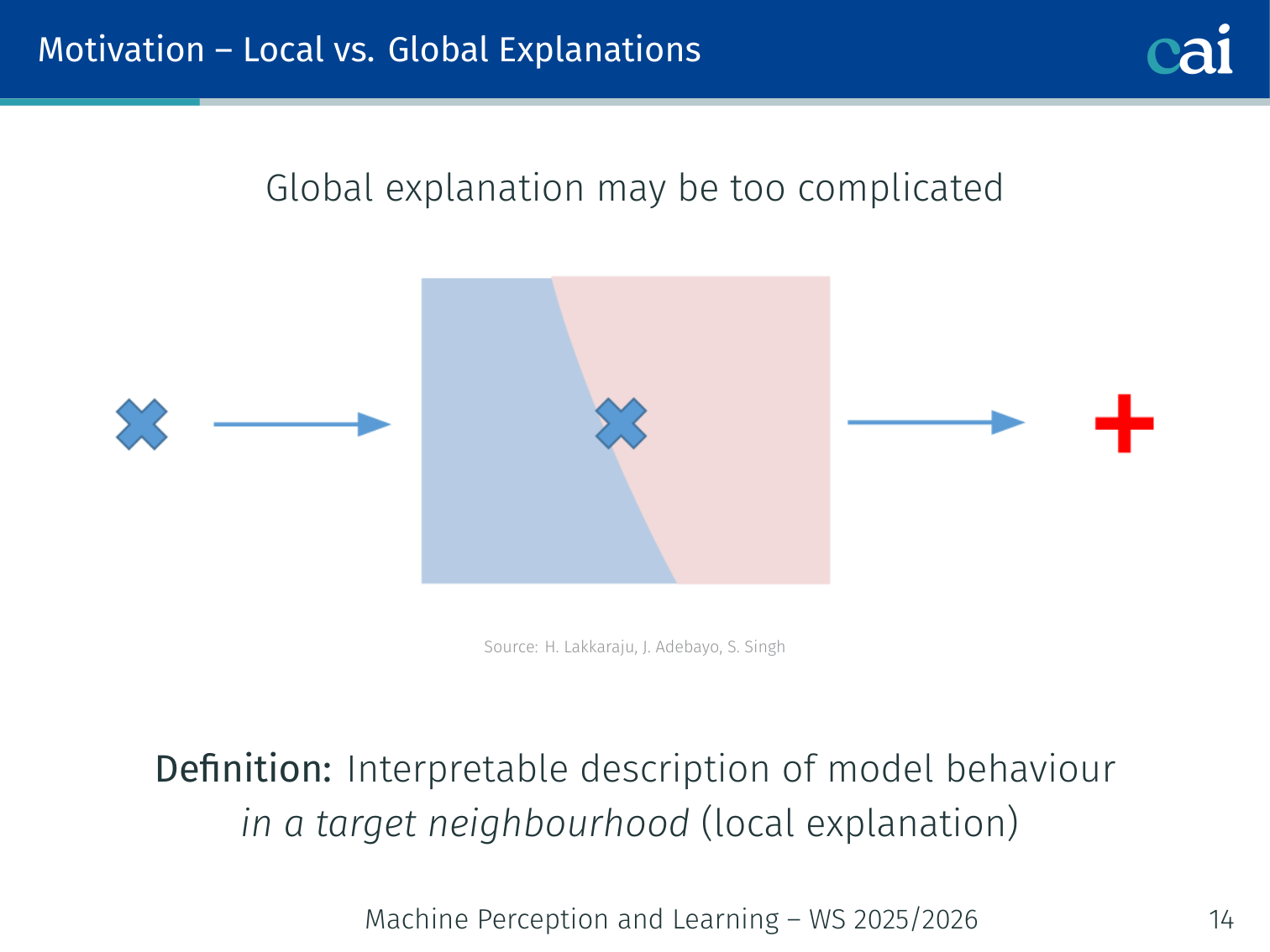
It's helpful to compare local explanations for one instance versus global ones for the whole model.

	Local	Global
Scope	One prediction	Entire model behaviour
Use case	Verify an individual decision is made for the right reasons	Detect big-picture biases across subgroups; vet for deployment
Definition	Interpretable description of model behaviour in a target neighbourhood	Interpretable description of complete model behaviour

---

Taxonomy of Post-hoc Explanation Methods

Post-hoc Explainability
├── Local
│   ├── Feature importances (LIME, SHAP)
│   ├── Rule-based (Anchors)
│   ├── Saliency maps (Input gradient, Grad-CAM, LRP, ...)
│   ├── Prototypes / Example-based (influence functions, activation maximisation)
│   └── Counterfactuals
└── Global
    ├── Collection of local explanations (SP-LIME)
    ├── Representation-based (Network Dissection, TCAV)
    └── Model distillation / summaries of counterfactuals

---

Feature Importances — LIME

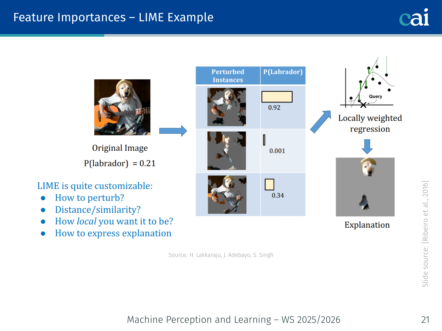
LIME basically builds a simple, local model to approximate how the big black box is behaving.

Authors: Ribeiro et al. (2016)

Key idea: Approximate the model locally around one prediction with a simple, sparse linear model. Being model-agnostic means it works on any black-box without requiring access to internals.

Algorithm

1. Given input $x$, generate $N$ perturbed variants by randomly masking features (superpixels for images, words for text, values for tabular data)
2. Query the black-box for predictions on all $N$ variants
3. Weight each variant by its proximity to $x$
4. Fit a weighted sparse linear model on (variants, predictions)
5. Linear model coefficients = feature importances for this prediction

import lime
import lime.lime_image
from skimage.segmentation import mark_boundaries
 
explainer = lime.lime_image.LimeImageExplainer()
explanation = explainer.explain_instance(
    image,
    model.predict,          # any callable black-box
    top_labels=1,
    hide_color=0,
    num_samples=1000
)
image_exp, mask = explanation.get_image_and_mask(
    label=explanation.top_labels[0],
    positive_only=True,
    num_features=5,
    hide_rest=False
)

Wolf vs. Husky example: LIME shows the model highlights snow (background) rather than the animal’s body when classifying a wolf — revealing the spurious feature.

Properties:

• Model-agnostic, works on any black box
• Faithful only locally near $x$, not globally
• Explanations can be unstable: similar inputs may yield very different explanations due to random perturbation sampling

---

Rule-Based Explanations — Anchors

Anchors give us those "if-then" rules that act as sufficient conditions for a prediction.

Check out these anchor examples—they're basically high-precision rules for specific local areas.

Authors: Ribeiro et al. (2018)

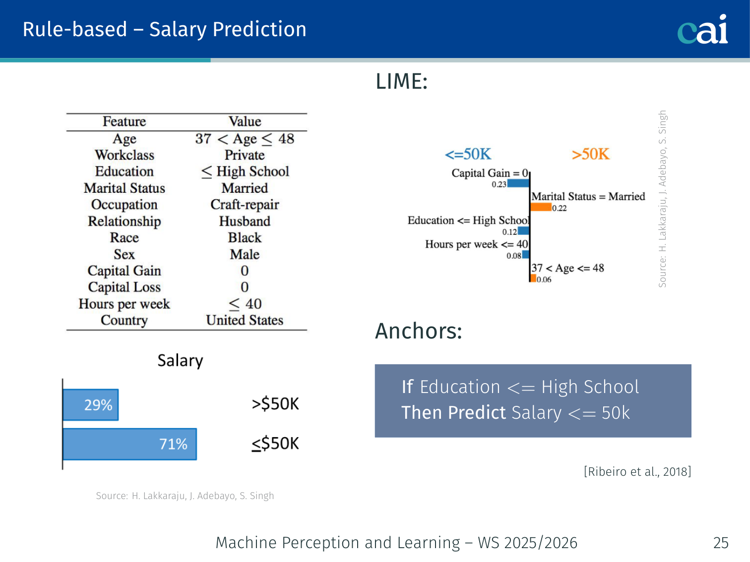
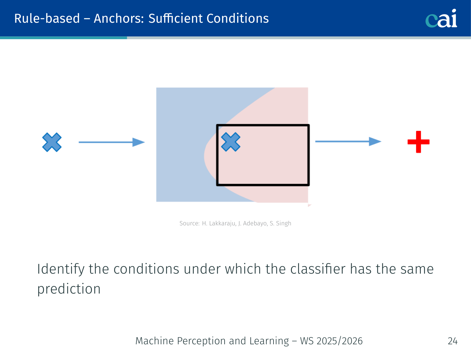
Anchors answer a different question from LIME: instead of “what features were most important?”, they ask “what is a sufficient condition for this prediction?”

Definition: An anchor is a rule such that the model’s prediction is the same (with high probability) whenever the rule holds, regardless of what the rest of the features are.

Salary prediction example:

Method	Output
LIME	Feature weights — age: +0.3, education: +0.5
Anchors	Rule — If Education ≤ High School → Predict Salary ≤ 50k

The anchor is interpretable as a human-readable condition that reliably reproduces the model’s prediction in its neighbourhood.

---

Saliency Maps

Saliency maps are great for highlighting exactly which pixels or features the model is leaning on.

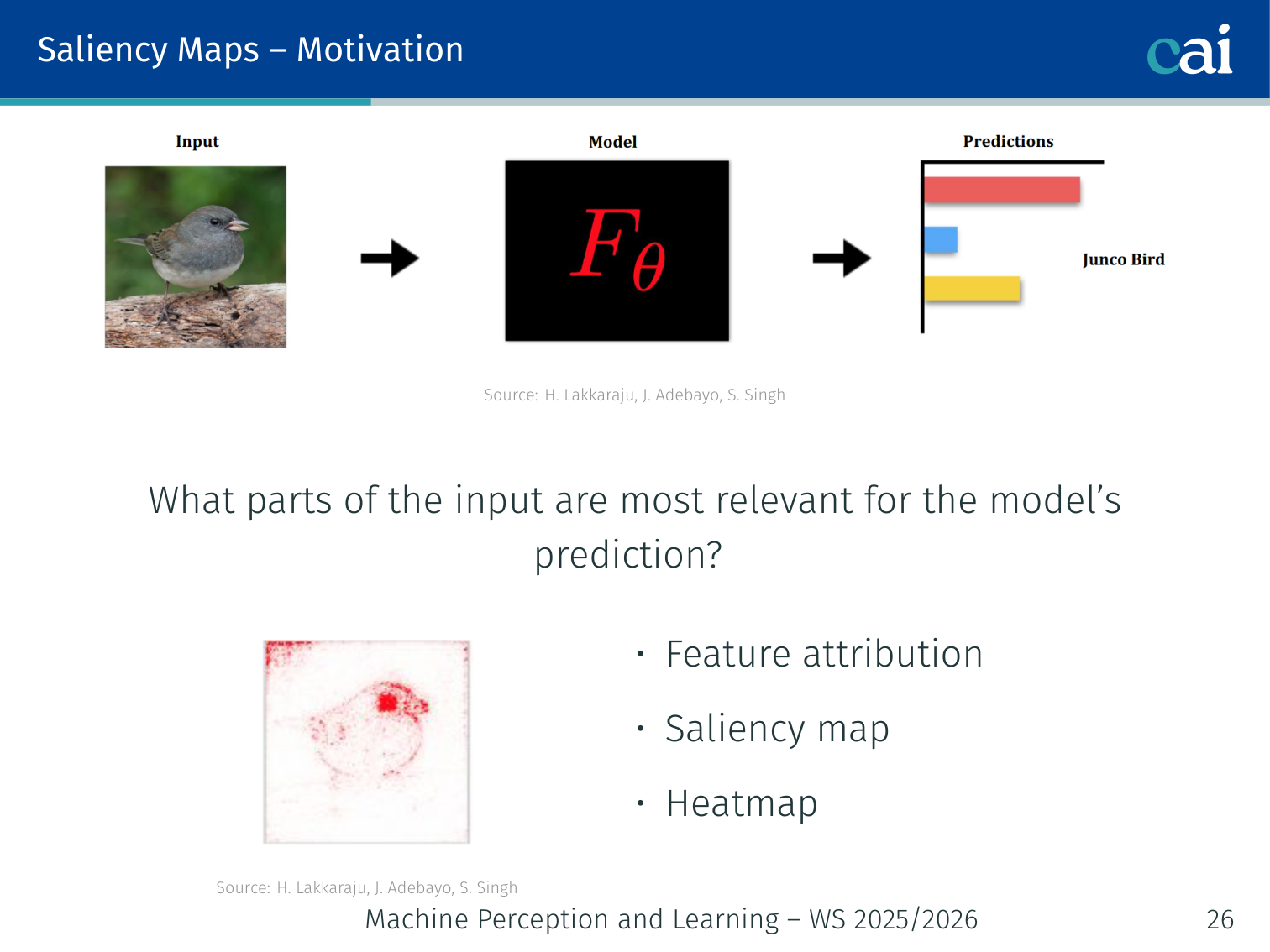
Heatmaps are a classic way to visualize which features are getting the most credit.

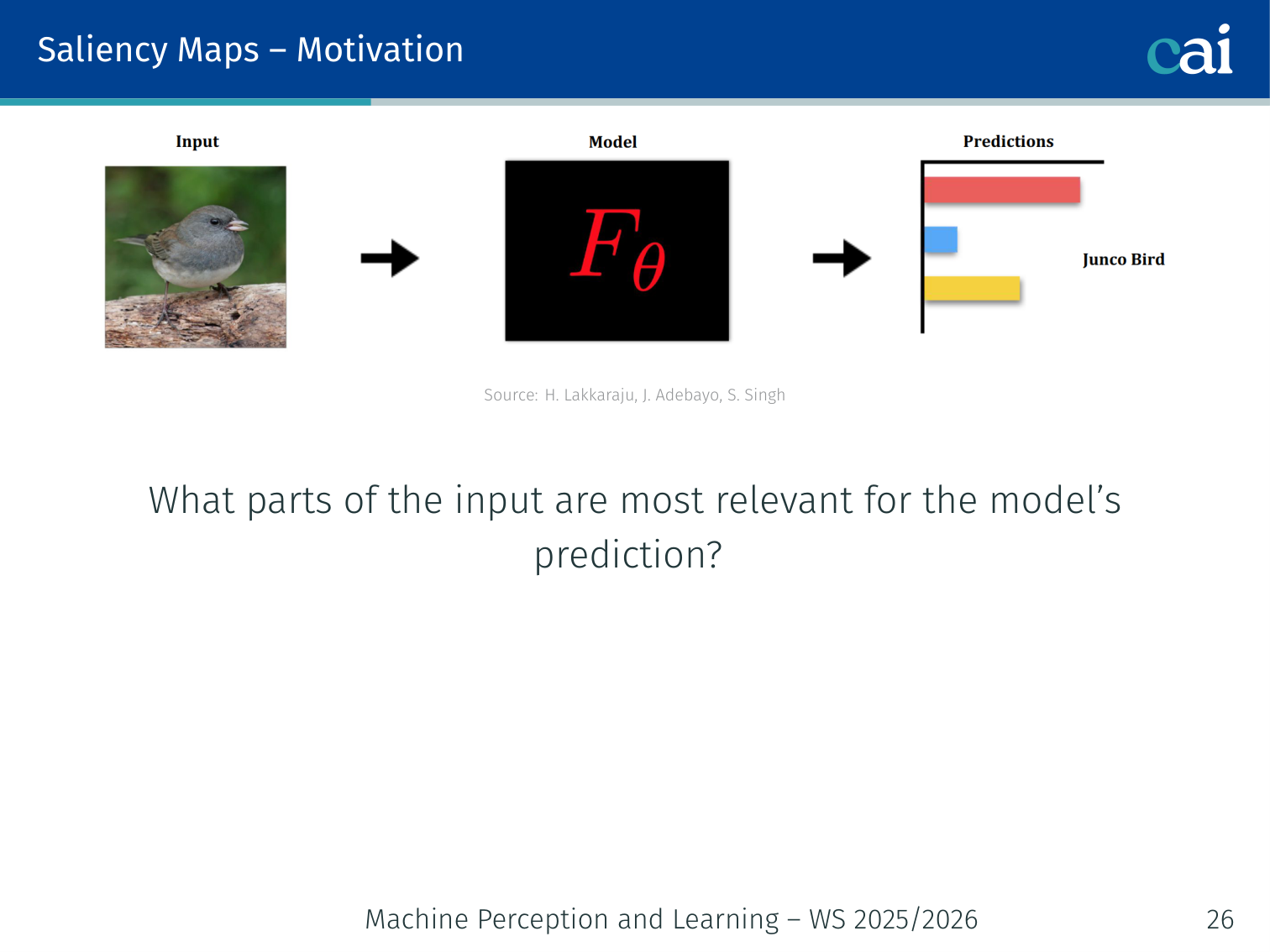
Saliency maps answer: “Which parts of the input were most relevant for the model’s prediction?”

Also called: feature attribution maps, heatmaps.

1. Input Gradient (Vanilla Saliency)

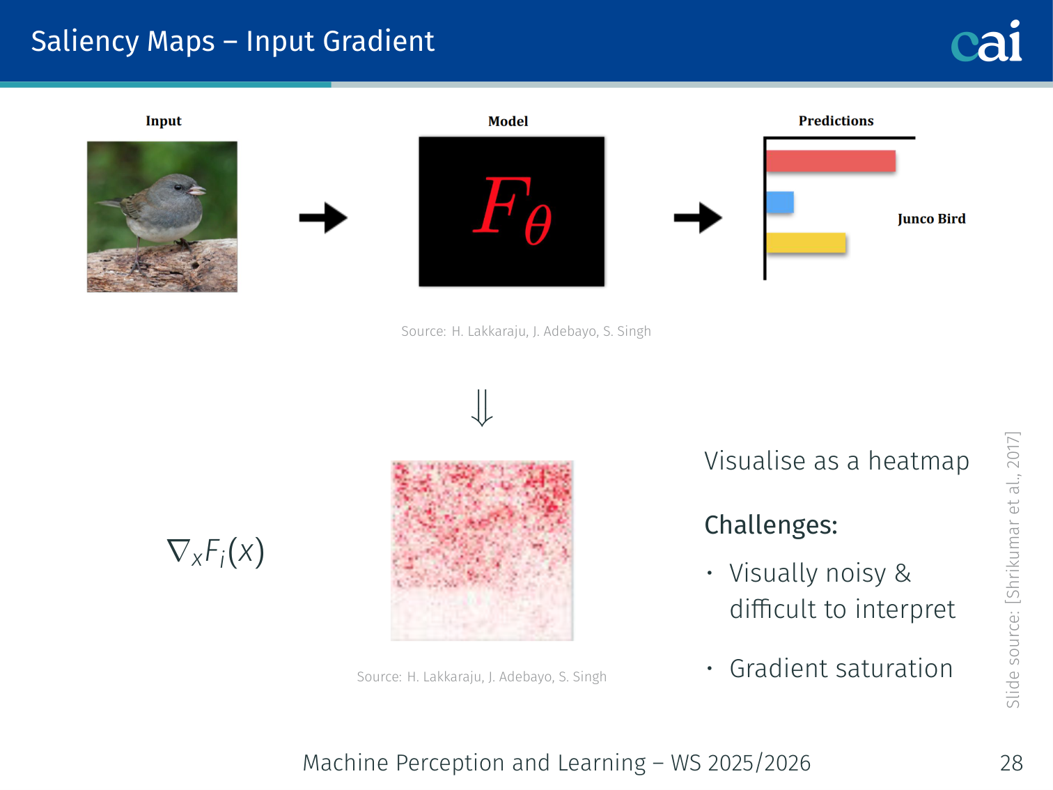
Vanilla saliency maps just look at the raw input gradients to see what's influential.

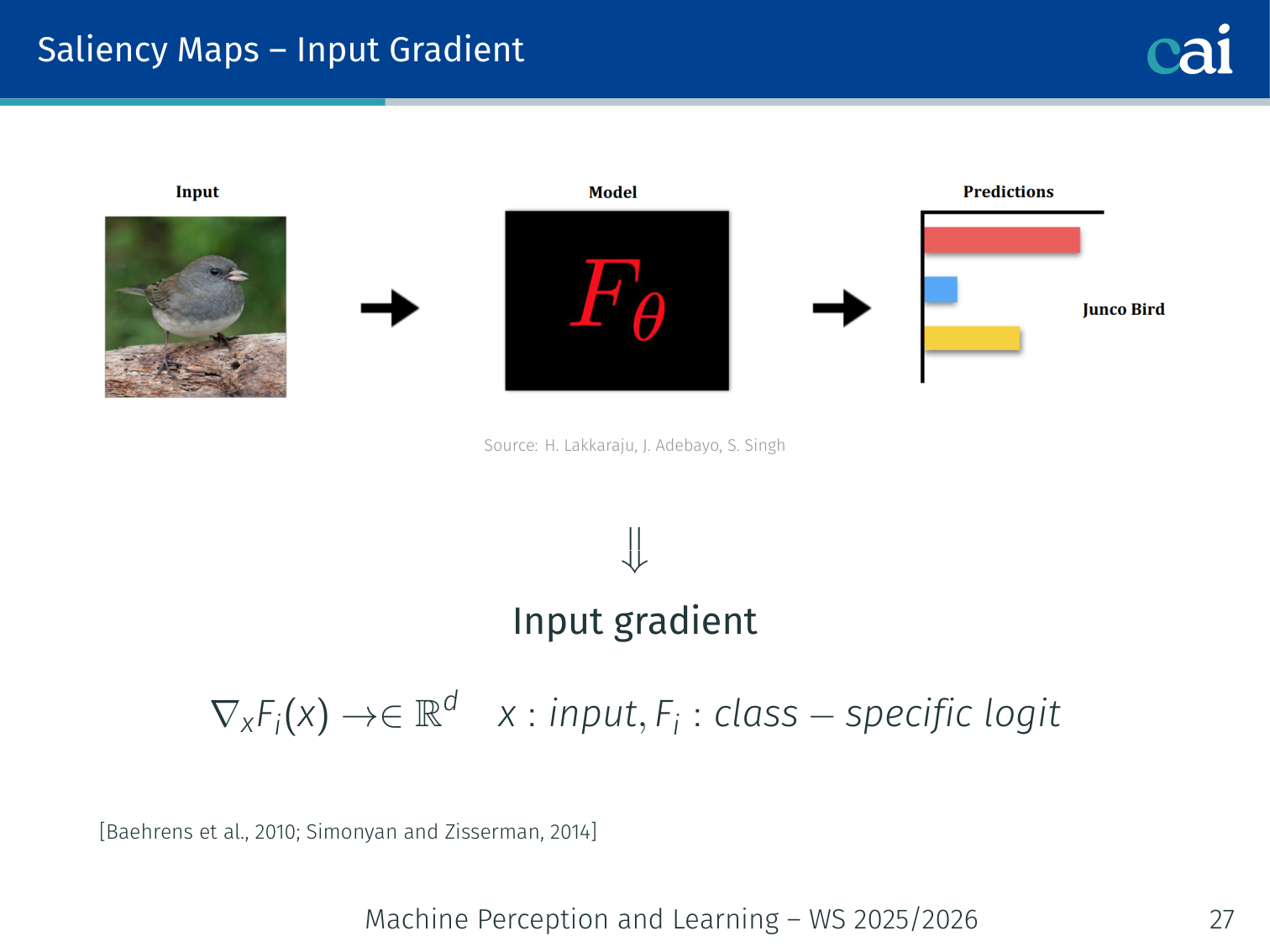
Using gradients is a direct way to see how much each feature contributes to the final score.

Compute the gradient of the class-specific logit $F_i(x)$ with respect to the input $x$:

$\text{Saliency}={\nabla }_x{F}_i(x)\in {\mathbb{R}}^d$

Visualise as a heatmap. Large magnitude = high influence.

model.eval()
x.requires_grad_(True)
output = model(x)
output[0, target_class].backward()
saliency = x.grad.data.abs().max(dim=0).values  # collapse channels

Challenges:

• Visually noisy and hard to interpret
• Gradient saturation: in flat regions of the loss landscape, gradients vanish even when the feature truly matters

2. SmoothGrad

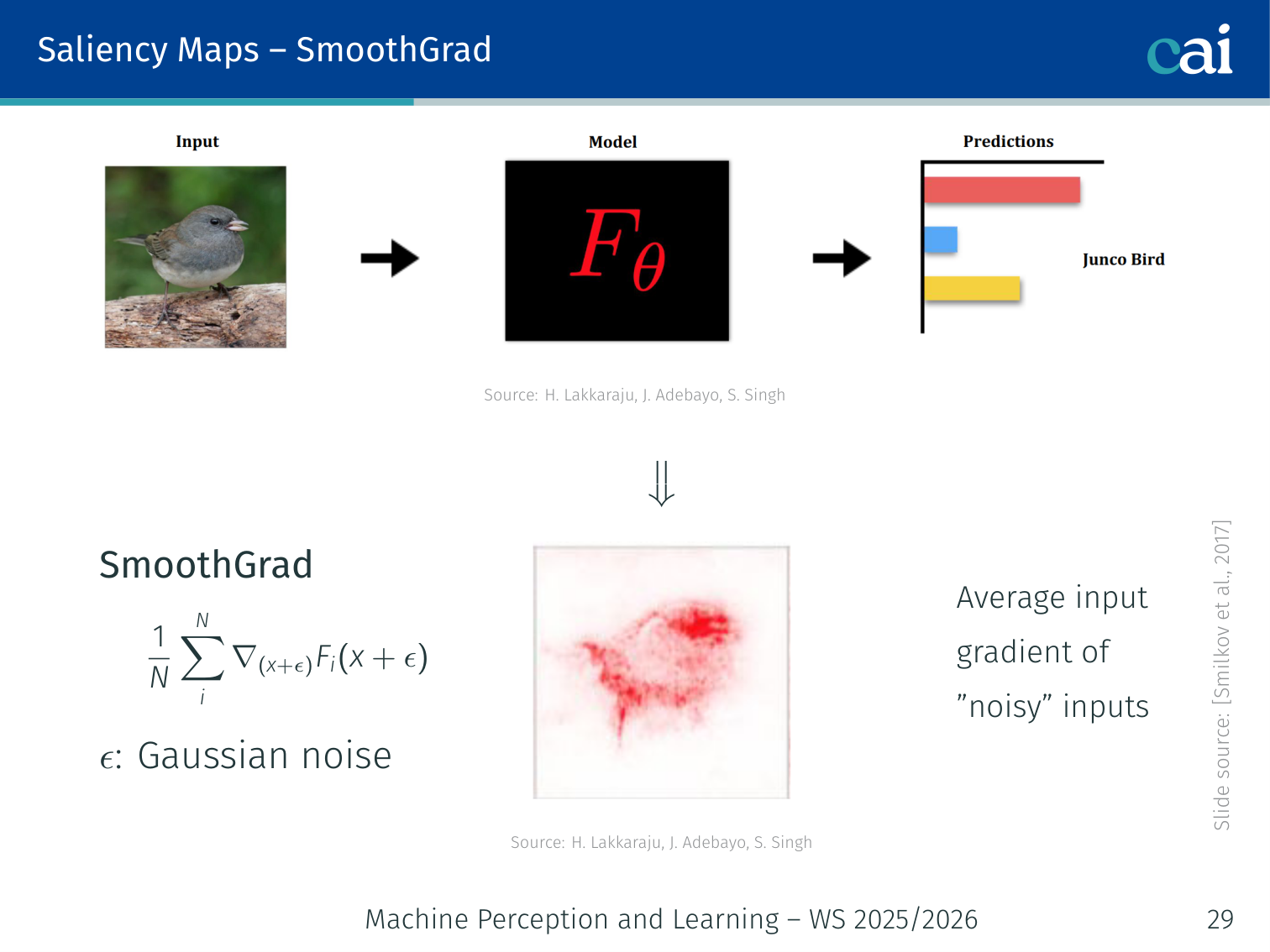
SmoothGrad helps clean things up by averaging the gradients over some noisy copies of the input.

Average the input gradient over $N$ noisy copies of the input to reduce noise:

$\text{SmoothGrad}(x)=\frac{1}{N}{\sum }_{i=1}^N{\nabla }_{x+{ϵ}_i}F(x+{ϵ}_i)$

where ${ϵ}_i\sim \mathcal{N}(0,{\sigma }^2)$. Produces cleaner, more interpretable maps.

3. Integrated Gradients

Integrated Gradients is a bit more robust—it avoids saturation and satisfies that completeness axiom.

Vanilla input gradients only measure the local slope at the input $x$. This creates a problem in saturated regions: the gradient can be near zero even when a feature was crucial for the prediction. Integrated Gradients was proposed to address this and to satisfy the completeness axiom, i.e. the attributions should sum to the prediction difference between the input and a baseline (Sundararajan et al., 2017).

Given an input $x$, a baseline $x^{\prime }$, and model output $F(x)$, the attribution for feature $i$ is

$${\mathrm{IG}}_i(x)=(x_i-x_i^{\prime }){\int }_0^1\frac{\partial F(x^{\prime }+\alpha (x-x^{\prime }))}{\partial x_i}d\alpha$$

So instead of taking the gradient only at $x$, we integrate the gradient along the straight-line path from the baseline $x^{\prime }$ to the input $x$.

Riemann Sum Approximation

In practice, the integral is approximated numerically:

$${\mathrm{IG}}_i(x)\approx (x_i-x_i^{\prime })\frac{1}{m}\sum _{k=1}^m\frac{\partial F\left(x^{\prime }+\frac{k}{m}(x-x^{\prime })\right)}{\partial x_i}$$

A common default is $m=50$ steps.

Baseline Choice

The baseline represents “absence of signal”, but this depends on the task. Common image baselines are:

• black image
• blurred image
• random noise

The explanation can change significantly with the baseline, so this choice matters.

Example: For an image classifier, a black baseline asks: which pixels had to be added when moving from an empty image to this specific input in order to obtain the current prediction?

Captum Example

import torch
from captum.attr import IntegratedGradients
 
model.eval()
ig = IntegratedGradients(model)
 
attributions, delta = ig.attribute(
    x,
    baselines=torch.zeros_like(x),   # black image baseline
    target=target_class,
    n_steps=50,
    return_convergence_delta=True,
)
 
saliency = attributions.abs().sum(dim=1)  # collapse channels

Integrated Gradients is often more stable than vanilla gradients and, up to numerical approximation, satisfies

$$\sum _i{\mathrm{IG}}_i(x)\approx F(x)-F(x^{\prime })$$

which is the desired completeness property.

4. Gradient × Input

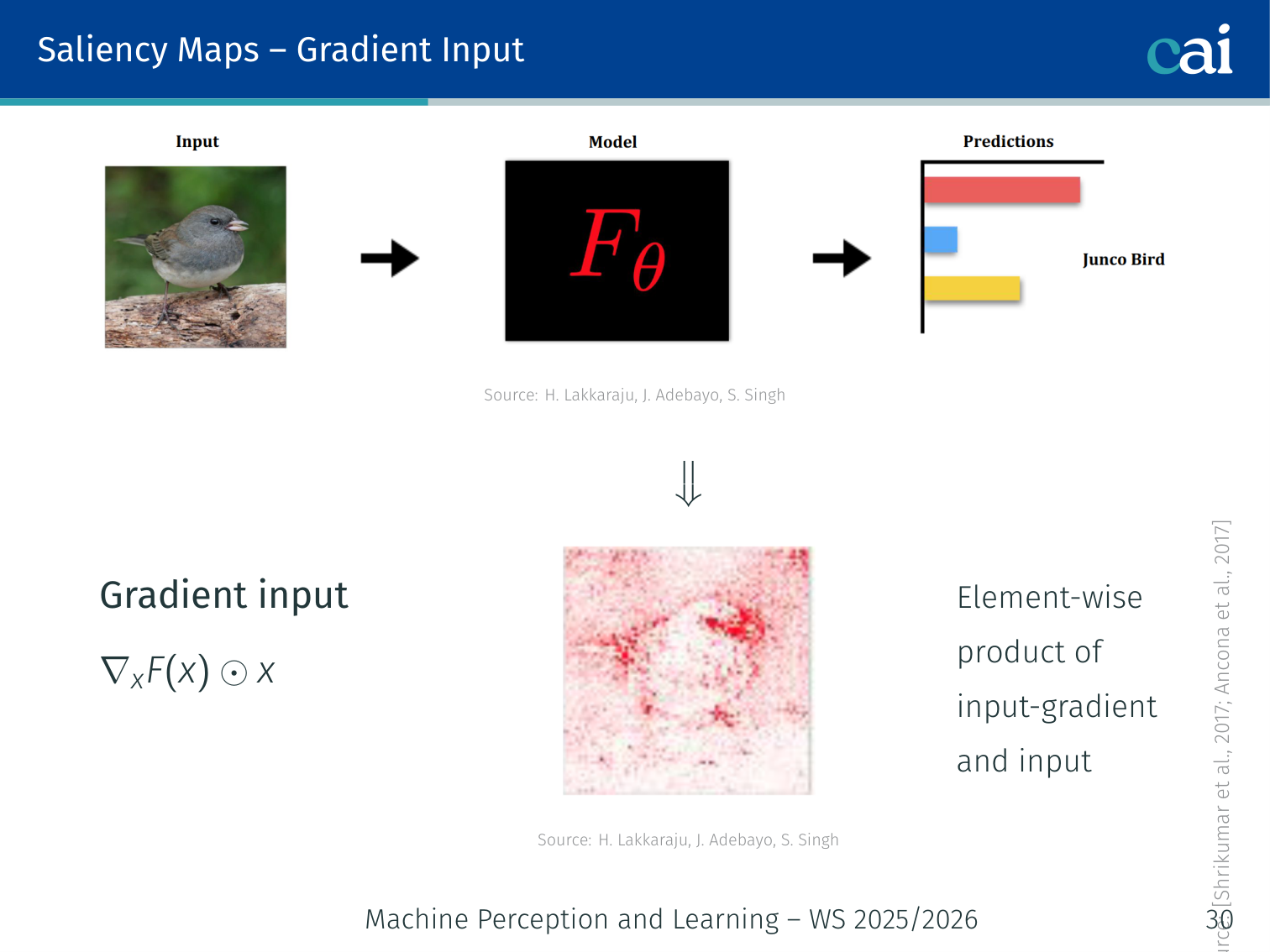
Multiplying the gradient by the input helps us account for the actual scale of each feature.

Element-wise product of the input gradient and the input itself:

$\text{GradInput}(x)={\nabla }_{x}F(x)\odot x$

Accounts for the magnitude of the input feature, not just its sensitivity.

5. Guided Backpropagation

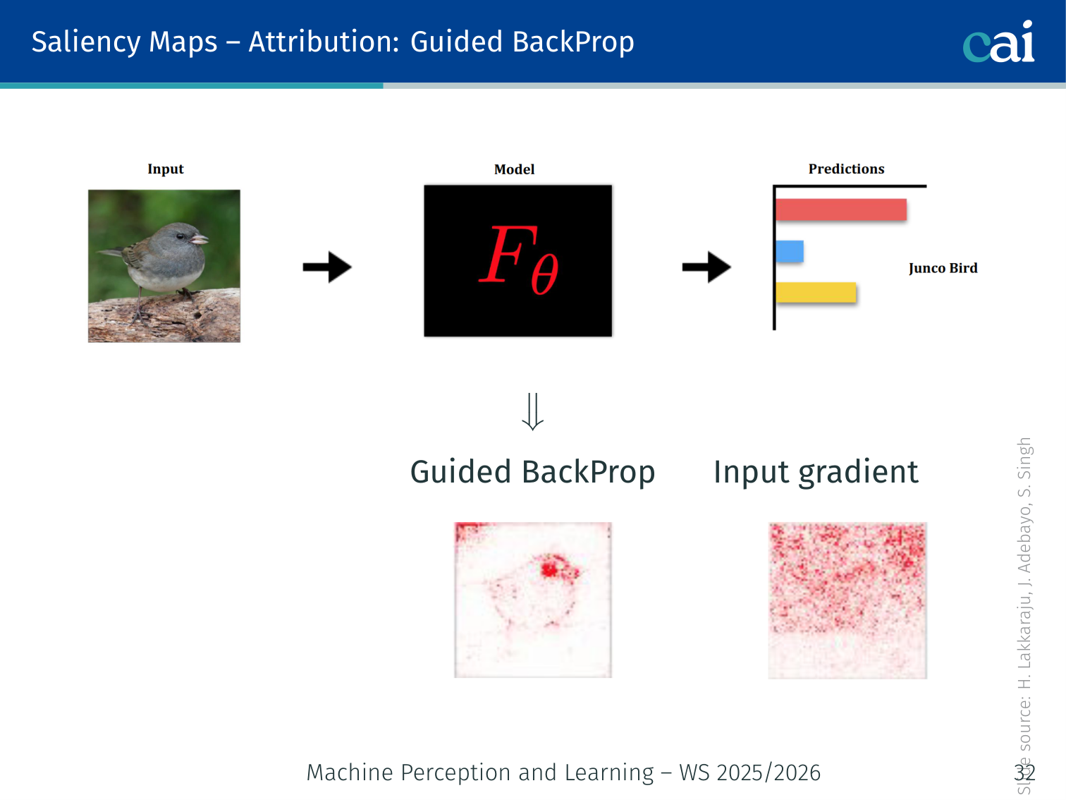
Guided Backprop gives us much sharper maps by being more selective about which gradients it passes back.

Modify the backward pass through ReLUs: zero out gradient entries that are either negative OR whose forward activation was negative:

$R_i^l=(f_i^l>0)\cdot (R_i^{l+1}>0)\cdot R_i^{l+1}$

This produces sharper, less noisy maps compared to vanilla gradients.

6. Layer-wise Relevance Propagation (LRP)

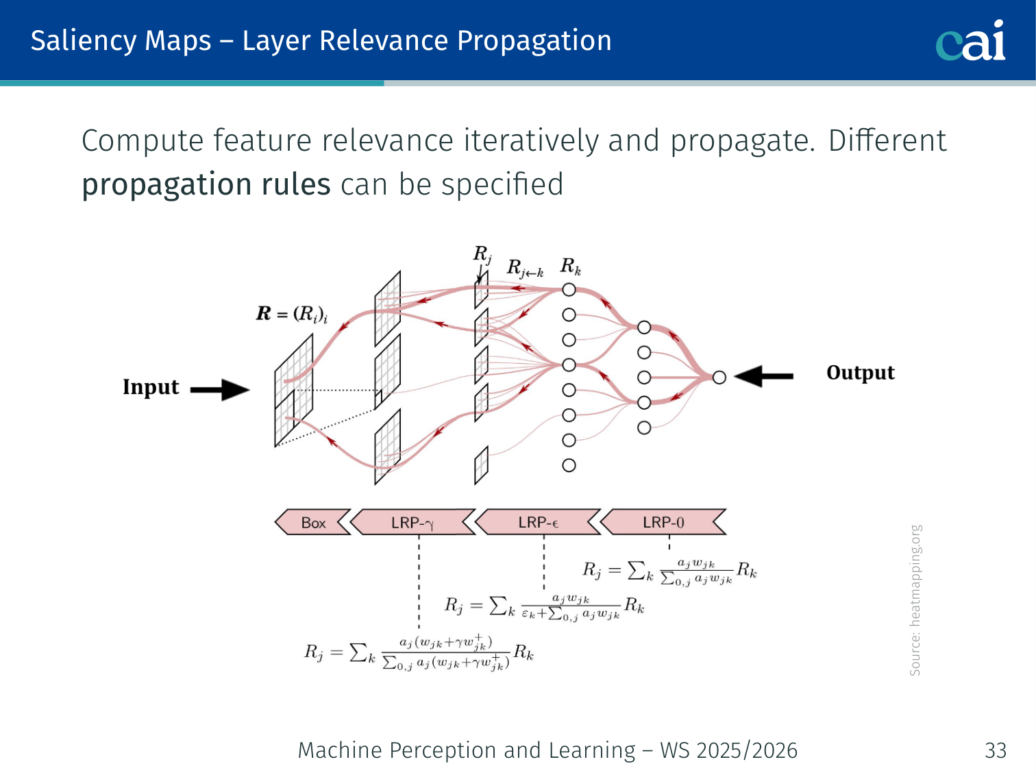
LRP is all about redistributing the output score back through the layers in a conservative way.

Propagate a “relevance” score from the output back through the network iteratively, using conservation rules. Different propagation rules can be specified per layer type. Heatmapping.org provides visualisations.

7. Grad-CAM

Authors: Selvaraju et al. (2017)

Grad-CAM produces a spatial heatmap showing which regions of the image mattered, using the last convolutional layer’s feature maps.

Algorithm:

1. Forward pass → feature maps $A^k$ at the last conv layer (shape $H^{\prime }\times W^{\prime }\times K$)
2. Compute gradient of class $c$ score w.r.t. feature maps: $\frac{\partial y^c}{\partial A_{ij}^k}$
3. Global average pool the gradients → importance weight per channel: ${\alpha }_k^c=\frac{1}{Z}{\sum }_i{\sum }_j\frac{\partial y^c}{\partial A_{ij}^k}$
4. Weighted combination + ReLU (keep only positive contributions to class $c$): ${\text{Grad-CAM}}^c=\text{ReLU}\left({\sum }_k{\alpha }_k^c{A}^k\right)$
5. Upsample to input image size → overlay as heatmap

def grad_cam(model, x, target_class):
    features, grads = None, None
 
    def fwd(m, inp, out):
        nonlocal features; features = out
    def bwd(m, gi, go):
        nonlocal grads; grads = go[0]
 
    h_f = model.layer4.register_forward_hook(fwd)
    h_b = model.layer4.register_backward_hook(bwd)
 
    model(x)[0, target_class].backward()
    weights = grads.mean(dim=(2, 3), keepdim=True)
    cam = (weights * features).sum(1).relu()
    cam = F.interpolate(cam.unsqueeze(1), x.shape[-2:], mode='bilinear')
 
    h_f.remove(); h_b.remove()
    return cam

Variants:

Variant	Improvement
Grad-CAM++	Better localisation when multiple instances of a class exist
Score-CAM	Perturbation-based, no gradients needed
Guided Grad-CAM	Combines Grad-CAM with Guided Backprop for pixel-precise detail

Additional saliency methods: CAM [Zhou et al., 2016], Meaningful Perturbation [Fong & Vedaldi, 2017], RISE [Petsiuk et al., 2018], DeepLIFT [Shrikumar et al., 2017], Expected Gradients [Erion et al., 2019].

---

Prototypes / Example-based Explanations

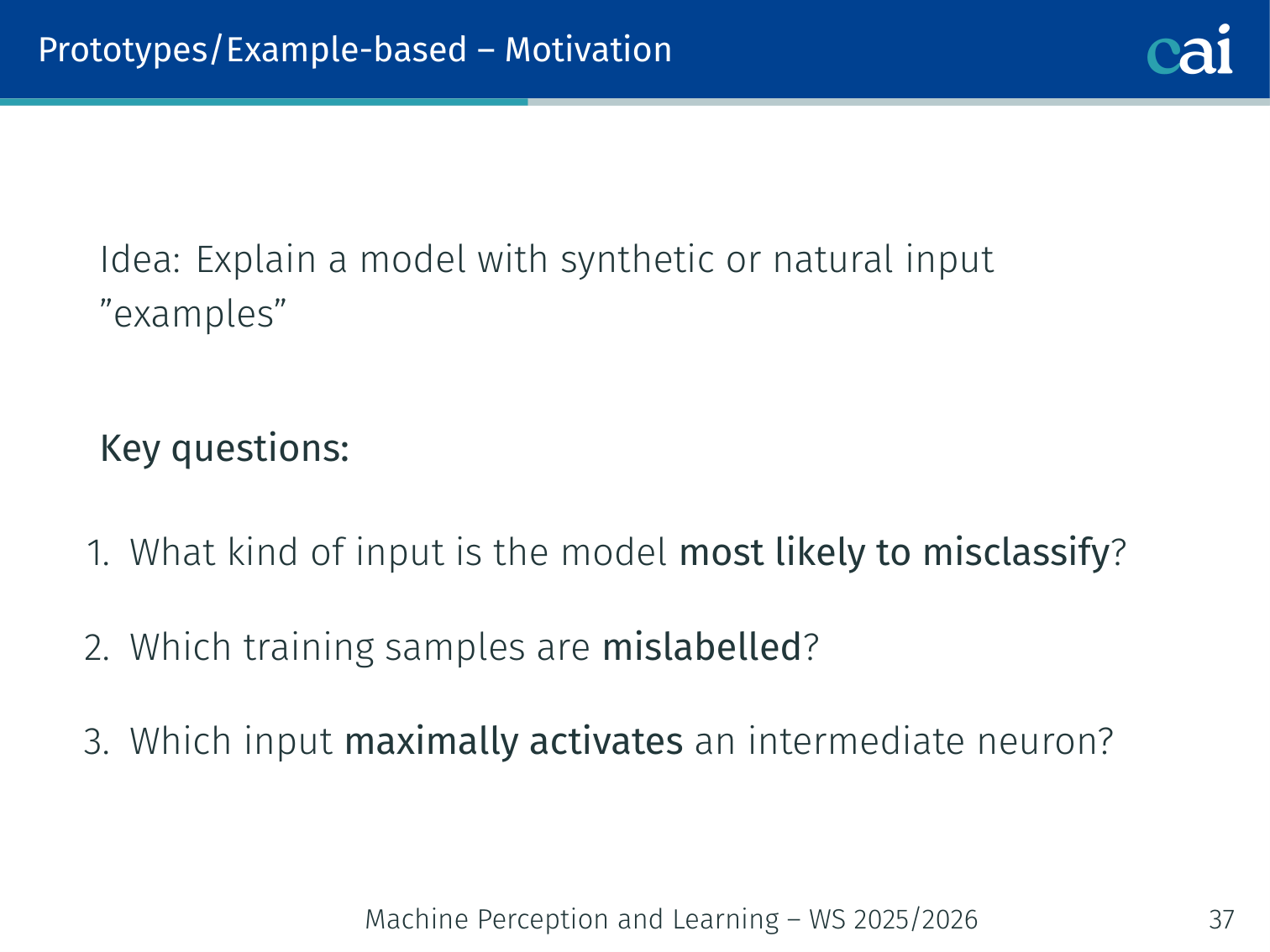
Sometimes it's easier to explain things using actual examples, like prototypes or influential samples from the training set.

Key idea: Explain a model not with feature weights but with example inputs — real or synthetic — that illuminate its behaviour.

Key questions:

1. Which training samples maximally influence the test loss?
2. Which inputs are the model most likely to misclassify?
3. Which input maximally activates a given internal neuron?

Influence Functions [Koh & Liang, 2017]

Identify which training examples had the most influence on a given test prediction.

Example: For a misclassified test image, the most influential training sample might be a mislabelled image with a very similar appearance — explaining why the model was confused.

Activation Maximisation / Feature Visualisation

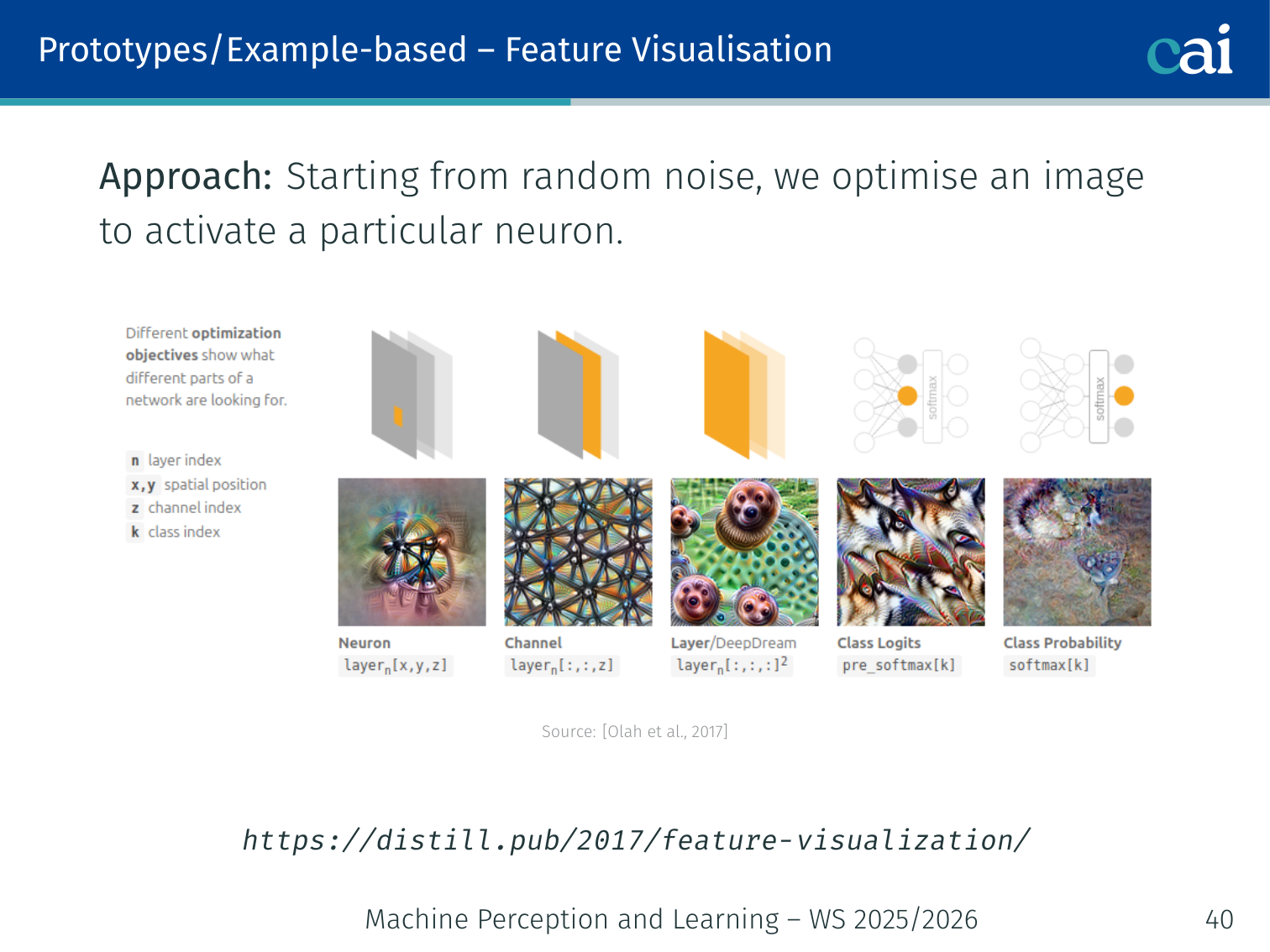
We can visualize what a neuron likes by optimizing an image to maximize its activation.

Starting from random noise, optimise an image via gradient descent to maximally activate a specific neuron or class output [Olah et al., 2017]:

$x^{\ast }=\arg {\max }_x{f}_k(x)-\lambda \Vert x{\Vert }^2$

# Maximise activation of neuron k in a target layer
x = torch.randn(1, 3, 224, 224, requires_grad=True)
optimizer = torch.optim.Adam([x], lr=0.1)
 
for step in range(500):
    optimizer.zero_grad()
    activation = model.features(x).mean()   # target neuron/layer
    loss = -activation + 1e-4 * x.norm()    # regularise to avoid noise
    loss.backward()
    optimizer.step()

This reveals what concept each neuron is detecting. See [distill.pub/2017/feature-visualization] for examples at scale.

---

Counterfactual Explanations

Key question: “What is the minimum change to the input to flip the model’s decision?”

This provides recourse — actionable feedback to individuals affected by a model’s decision.

Example: “Your loan application was denied. If you increased your annual income by €15K and paid your credit card bills on time for three months, it would be approved.”

Counterfactuals are fundamentally different from saliency: saliency says “this feature mattered”; counterfactuals say “change this feature to get a different outcome”.

1. Minimum Distance Counterfactuals [Wachter et al., 2017]

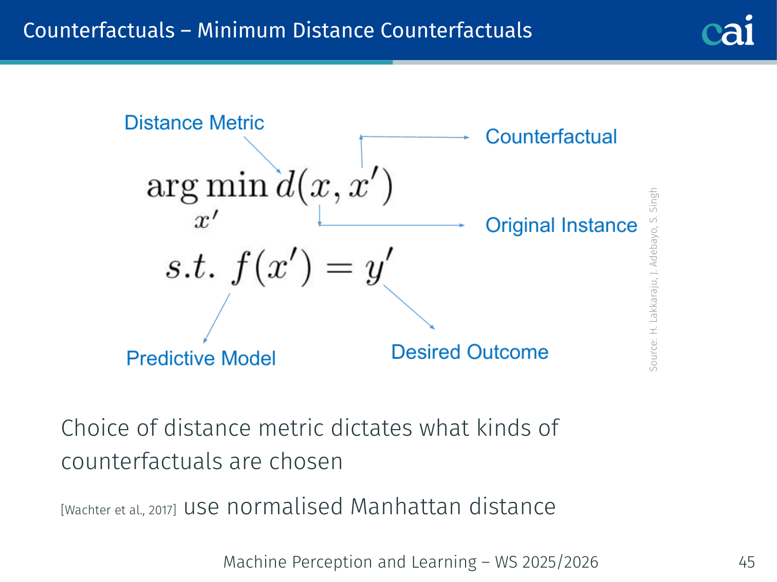
Minimum distance counterfactuals tell you the smallest change needed to flip the outcome—super useful for recourse.

$x^{CF}=\arg {\min }_{x^{\prime }}d(x,x^{\prime })\text{s.t.}f(x^{\prime })=y^{\prime }$

Using normalised Manhattan distance penalises the total number of changes, favouring small perturbations over many large ones. The candidate CF1 vs. CF2 choice depends on which direction $A$ or $B$ you move $x$ along — the metric governs this.

2. Feasible and Least-Cost Counterfactuals [Ustun et al., 2019]

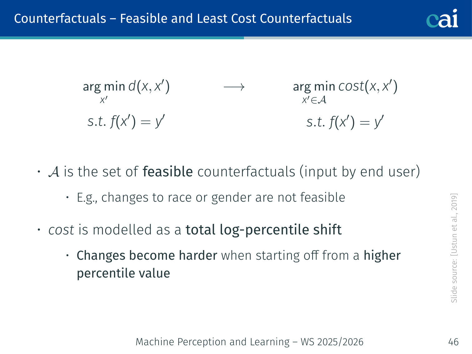
A bare minimum-distance counterfactual can suggest impossible changes (e.g., “change your race”). Adding actionability constraints:

$x^{CF}=\arg {\min }_{x^{\prime }\in \mathcal{A}}\text{cost}(x,x^{\prime })\text{s.t.}f(x^{\prime })=y^{\prime }$

• $\mathcal{A}$ = set of actionable counterfactuals (user-defined)
• Cost = total log-percentile shift (changes from a high percentile are more expensive)
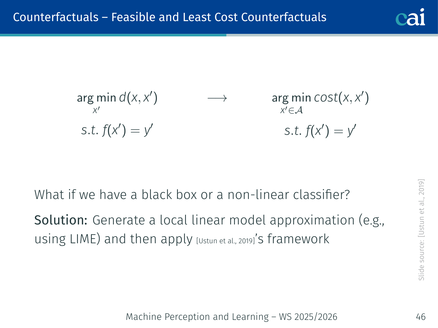
• For black-box or non-linear classifiers: generate a LIME local linear approximation first, then apply this framework

3. Causally Feasible Counterfactuals [Mahajan et al., 2019; Karimi et al., 2020]

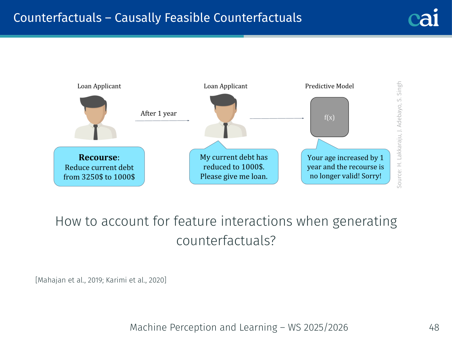
Changing one feature can be impossible without changing causally downstream features (e.g., changing income should also change debt-to-income ratio). Use a Structural Causal Model (SCM):

$x^{CF}=\arg {\min }_{x^{\prime }}{d}_{\text{causal}}(x,x^{\prime })\text{s.t.}f(x^{\prime })=y^{\prime }$

Implementation: solve via a variational autoencoder; requires access to model gradients. In practice, partial knowledge of the causal graph also works well.

4. Further Considerations

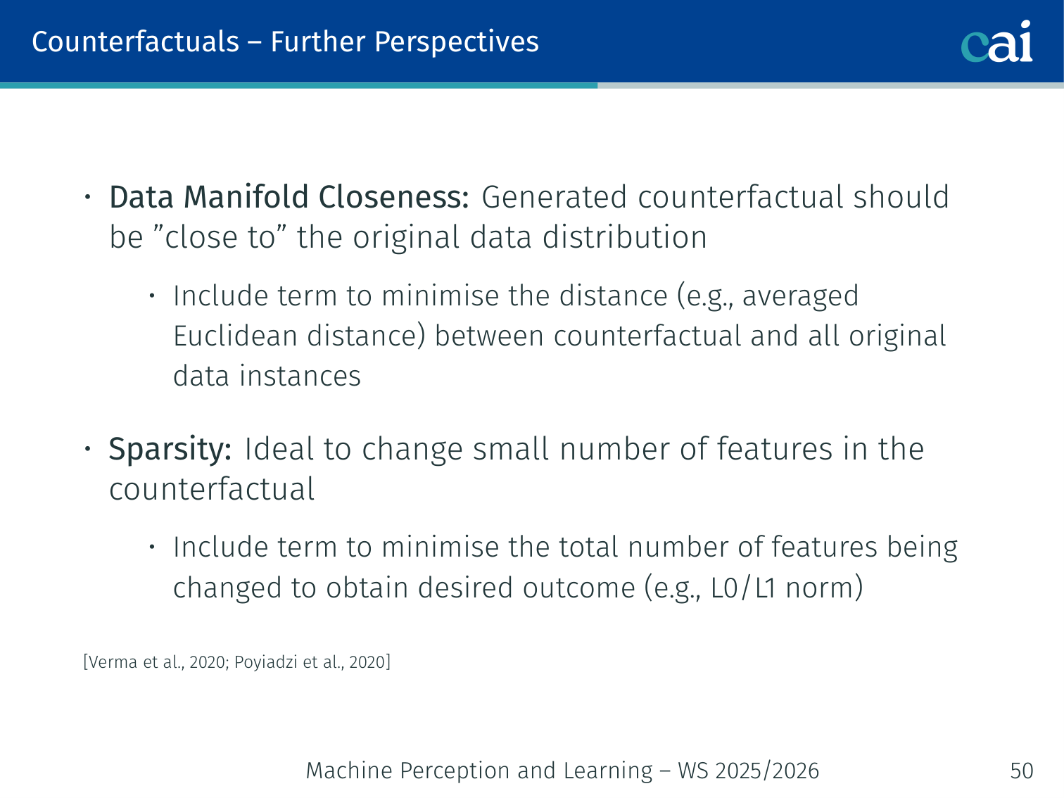
Consideration	Details
Data manifold closeness	Counterfactual should lie on the training distribution, not in an unrealistic region
Sparsity	Prefer counterfactuals that change few features (L0/L1 penalty on changed features)
Model access	Black-box vs. gradient-based → affects which algorithm to use

---

Global Explanations

Collection of Local Explanations — SP-LIME

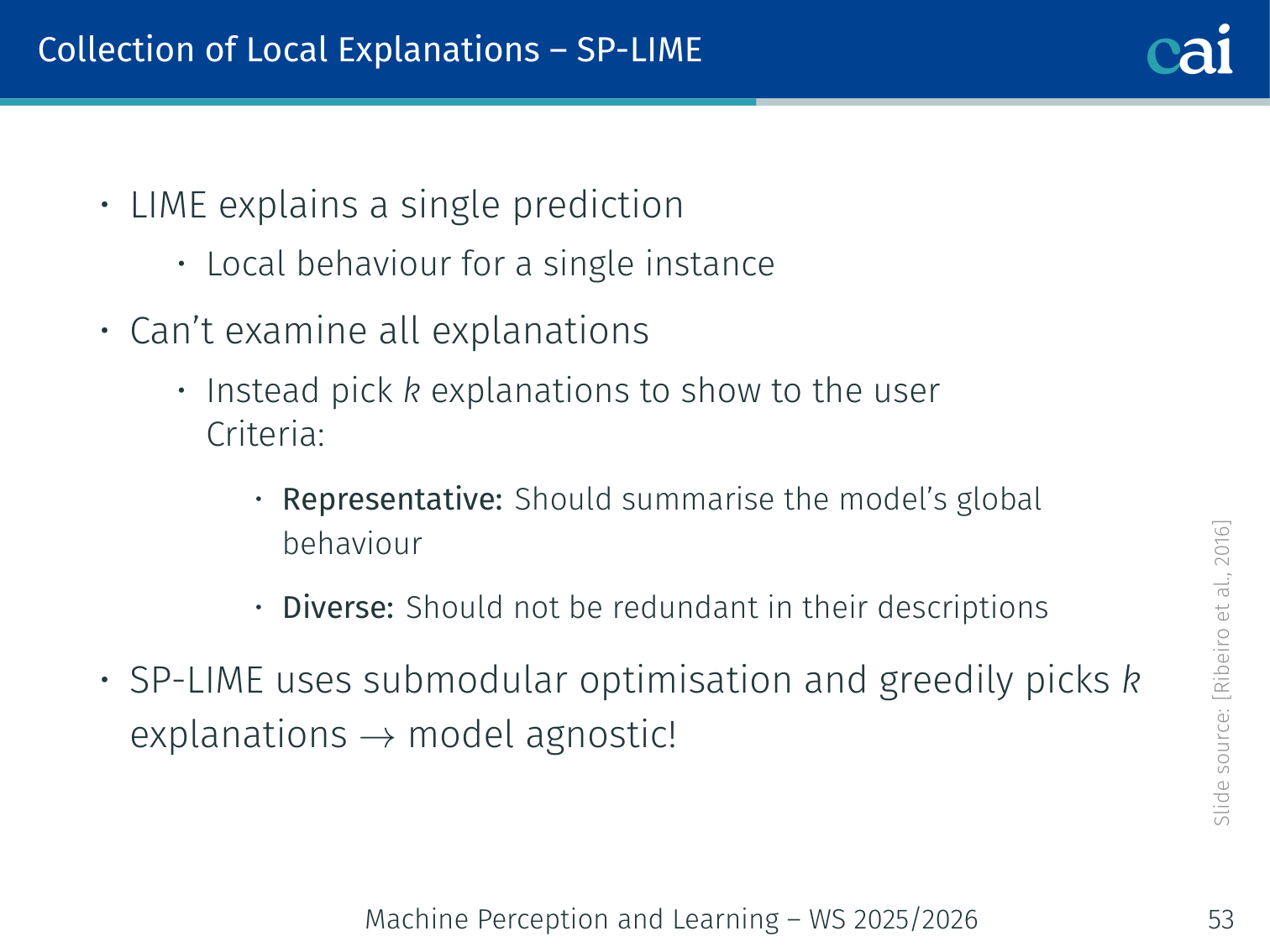
SP-LIME picks a representative set of local explanations to give you a global sense of the model.

Problem: LIME explains one prediction at a time. You can’t manually inspect thousands of local explanations.

SP-LIME (Submodular Pick LIME) selects $k$ representative and diverse local explanations to summarise the model’s global behaviour.

Criteria:

• Representative: the $k$ instances should collectively cover the most important features
• Diverse: explanations should not be redundant

Method: Greedy submodular optimisation over an explanation matrix (rows = instances, columns = features). Provably near-optimal and model-agnostic.

All instances → LIME for each → explanation matrix (N × F)
                                        ↓
                         Greedy submodular pick of k rows
                                        ↓
               k representative, diverse explanations shown to user

Representation-based — Network Dissection [Bau et al., 2017]

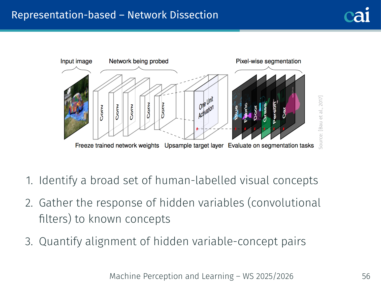
Network Dissection helps us map internal neurons to human-readable concepts like "stripes" or "wheels".

Determine what human-interpretable concepts are encoded by individual neurons (convolutional filters).

Procedure:

1. Collect a broad set of human-labelled visual concepts (colour, texture, part, scene, object)
2. For each concept, gather the response of every hidden unit (filter) to those concept examples
3. Quantify the alignment of each hidden unit–concept pair using IoU

Example: Filter 47 in layer conv5 may have IoU = 0.72 with the concept “wheel” — meaning this neuron consistently fires on wheels.

Representational Similarity

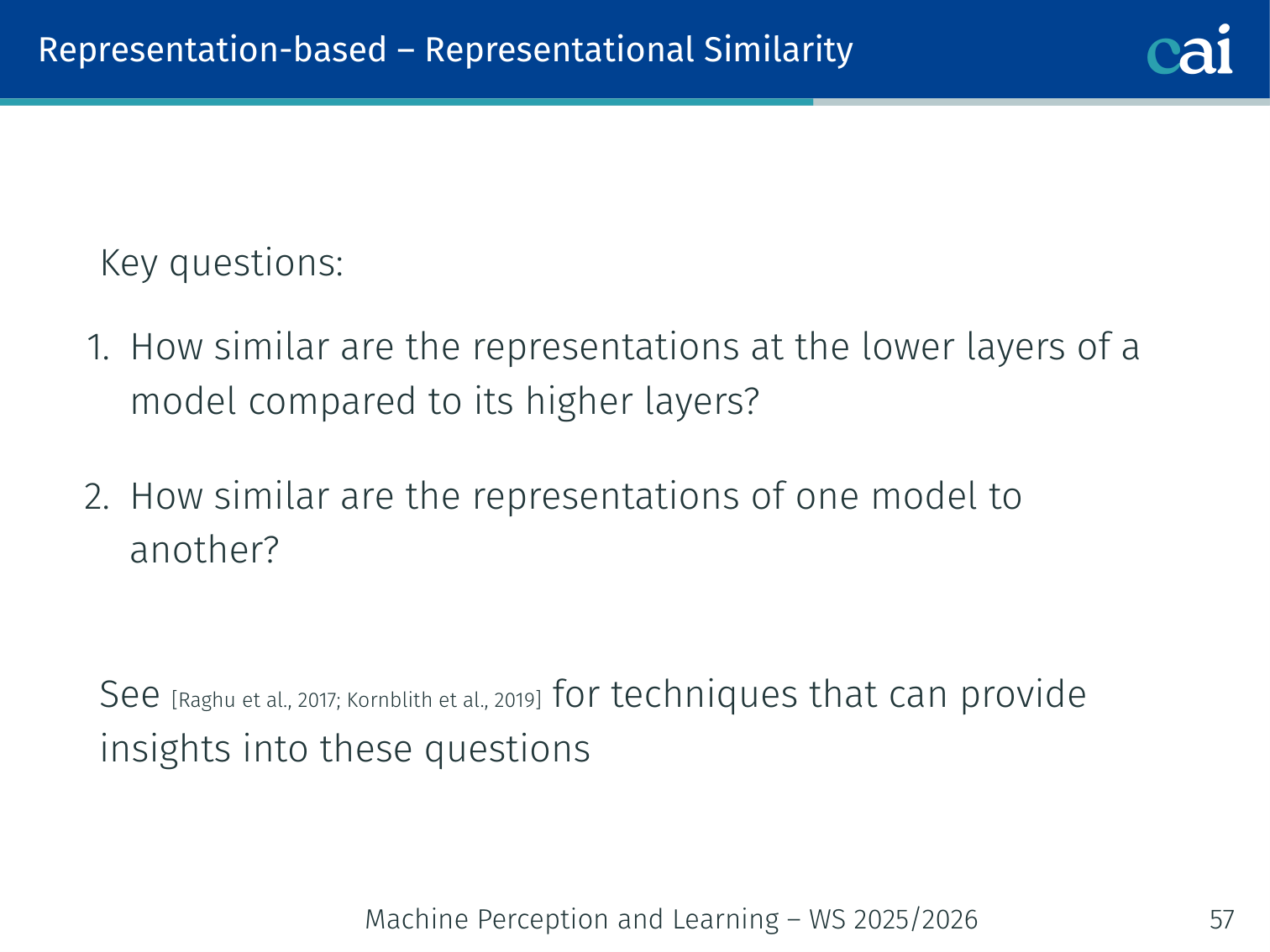
Checking representational similarity helps us see how different layers or models compare to each other.

Key questions: How similar are representations across layers of the same model? How similar are representations across different models?

See CKA [Kornblith et al., 2019] and SVCCA [Raghu et al., 2017] for techniques.

---

SHAP — SHapley Additive exPlanations

Authors: Lundberg & Lee (2017)

SHAP gives every feature a contribution score using Shapley values from cooperative game theory. The Shapley value of feature $i$ is its average marginal contribution across all possible orderings of features:

${\varphi }_i={\sum }_{S\subseteq F\setminus \{i\}}\frac{|S|!(|F|-|S|-1)!}{|F|!}[f(S\cup \{i\})-f(S)]$

Analogy: Features are players; the Shapley value is how much credit each player deserves for the team’s total score, averaged fairly over all possible coalition orderings.

Axiomatic Guarantees

Property	Meaning
Efficiency	${\sum }_i{\varphi }_i=f(x)-\mathbb{E}[f(x)]$ — values account for the full prediction
Symmetry	Features with equal contributions receive equal values
Dummy	Feature with zero marginal contribution → zero Shapley value
Linearity	Values are additive when games are combined

DeepSHAP

Approximates Shapley values for neural networks using backpropagation (combines DeepLIFT with SHAP theory):

import shap
import torchvision.models as models
 
model = models.vgg16(pretrained=True).eval()
# background = representative sample from training distribution
background = train_images[:50]
explainer = shap.DeepExplainer(model, background)
shap_values = explainer.shap_values(x_test)
shap.image_plot(shap_values, x_test)
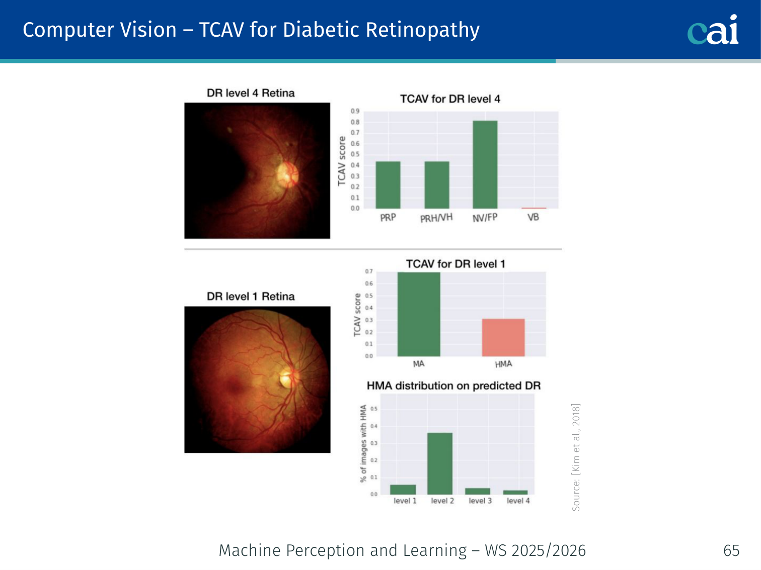
# Red pixels = pushed prediction toward class; blue = away

---

Concept-Based Explanations — TCAV

Authors: Kim et al. (2018)
TCAV = Testing with Concept Activation Vectors

Instead of per-pixel saliency, explain in terms of human-meaningful concepts (e.g., “striped texture”, “has ears”, “is green”).

Algorithm

1. Collect positive and negative examples for a concept $c$ (e.g., images with vs. without stripes)
2. Train a linear classifier on layer $l$‘s activations for those examples → the decision boundary direction is the Concept Activation Vector (CAV)
3. Compute the directional derivative of class $k$‘s output along the CAV direction
4. TCAV score = fraction of class $k$ inputs where moving along the CAV increases the class probability

${\text{TCAV}}_{k,c,l}=\frac{|\{x\in X_k:S_{k,c,l}(x)>0\}|}{|X_k|}$

# Pseudocode
cav_direction = train_cav_probe(concept_positives, concept_negatives, layer=l)
scores = []
for x in class_k_inputs:
    act = get_activations(model, x, layer=l)
    grad = get_class_gradient(model, x, class=k, layer=l)
    scores.append((grad @ cav_direction) > 0)
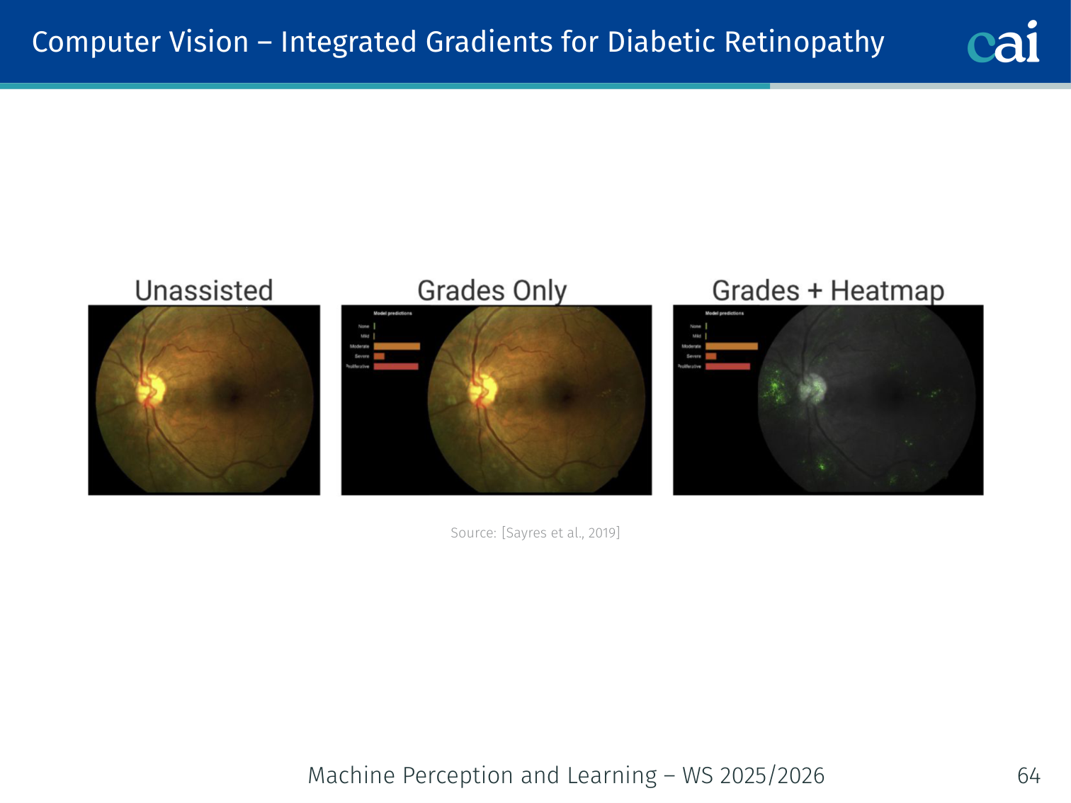
tcav_score = mean(scores)

Example — Diabetic Retinopathy diagnosis: A model’s TCAV scores might show it strongly relies on the concept “microaneurysms” (TCAV ≈ 0.85) and less on “general redness” (TCAV ≈ 0.4), aligning with clinical knowledge.

Example — Zebra classification: “Striped texture” scores TCAV ≈ 0.9, “has four legs” scores ≈ 0.4.

---

Probing Classifiers

Do the internal representations of a neural network encode specific concepts?

Train a linear probe on frozen layer $l$ representations to predict a human-defined concept:

text input → [Frozen BERT layer l] → linear probe → P(concept)

If a linear probe achieves high accuracy, the concept is linearly decodable from that layer’s representation.

Example: Train a probe on BERT layer 8 to predict part-of-speech tags. High accuracy → layer 8 encodes syntactic structure. Layer 12 probes for coreference tend to be more accurate than layer 2 probes, suggesting deeper layers encode more abstract structure.

---

Explanations in Different Modalities

Structured / Tabular Data

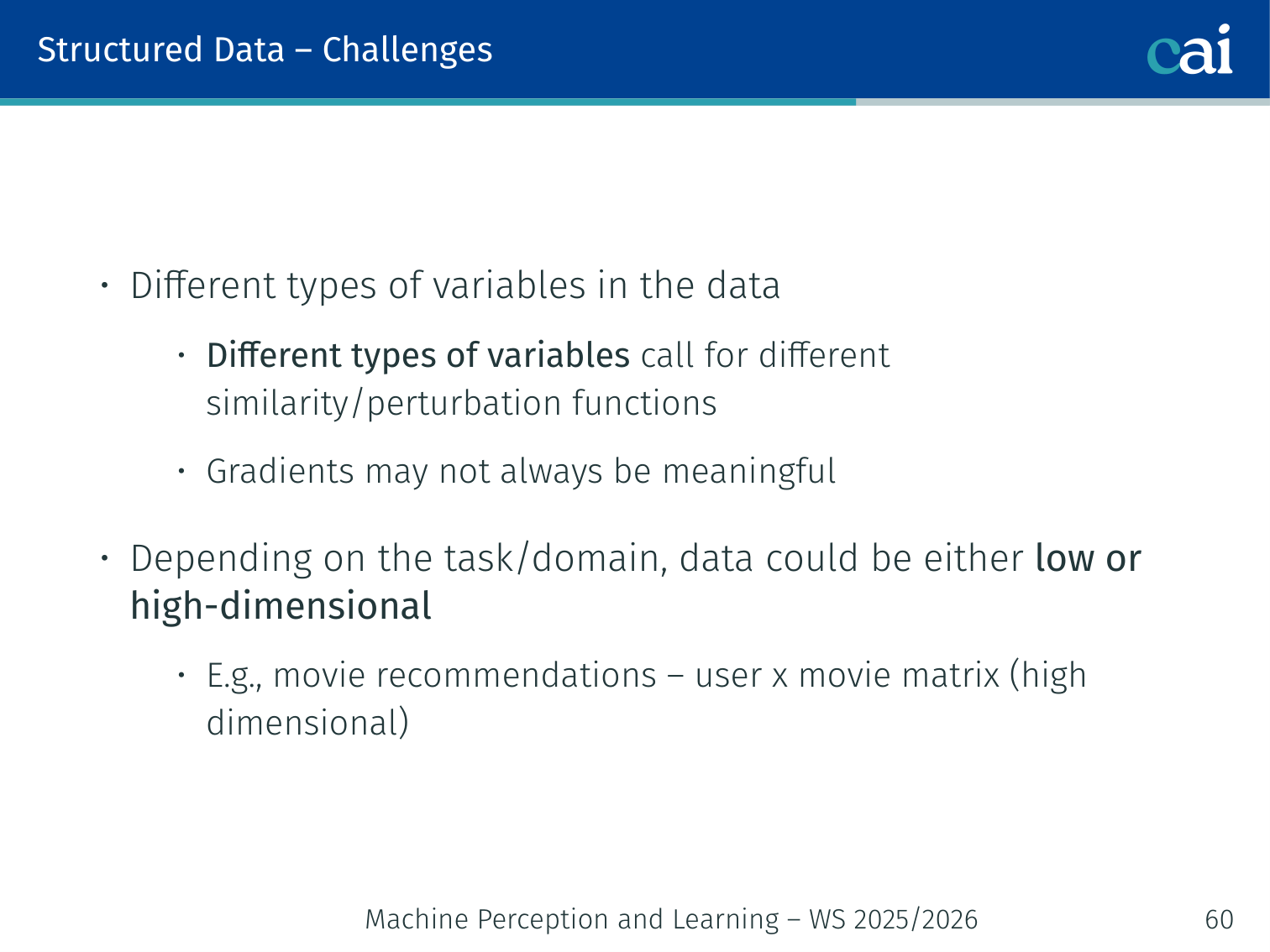
Explaining tabular data has its own set of challenges, like dealing with mixed types and discrete values.

Common in: disease diagnosis (weight, age, glucose), credit scoring (income, previous crimes), recommender systems.

Challenges:

• Mixed variable types (categorical, ordinal, continuous) require different similarity/perturbation functions
• Gradients may not be meaningful for discrete inputs
• Datasets can be very high-dimensional (e.g., a user × movie matrix)

Recommended methods: LIME, Anchors, rule-based explanations, counterfactuals. Saliency maps are generally not meaningful here.

Computer Vision

In computer vision, we have a ton of great tools for visualizing what the model sees.

Heatmaps and saliency maps help confirm if the model is focusing on the right visual cues.

Applicable methods: all gradient-based saliency (Input Gradient, Guided Backprop, Integrated Gradients, Grad-CAM), TCAV for concept-level explanations.

Example — Bone age prediction: Integrated gradients on an X-ray highlights the growth plates of the wrist bones — the same regions a radiologist would examine. TCAV for diabetic retinopathy confirms the model focuses on retinal microaneurysms.

Natural Language Processing

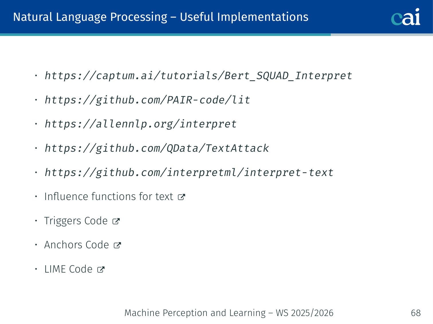
NLP is trickier because of the discrete nature of text, but we still have some solid interpretability methods.

Challenges:

• Discrete input space: gradients not directly applicable or interpretable
• Not all token-substitution perturbations are grammatical or meaningful
• Task format varies: classification, span selection, text generation

Useful tools: Captum, LIT (Language Interpretability Tool), AllenNLP Interpret, TextAttack, Anchors, LIME for text.

---

Evaluation of Explanations

At the end of the day, we need to evaluate whether these explanations are actually helpful for humans.

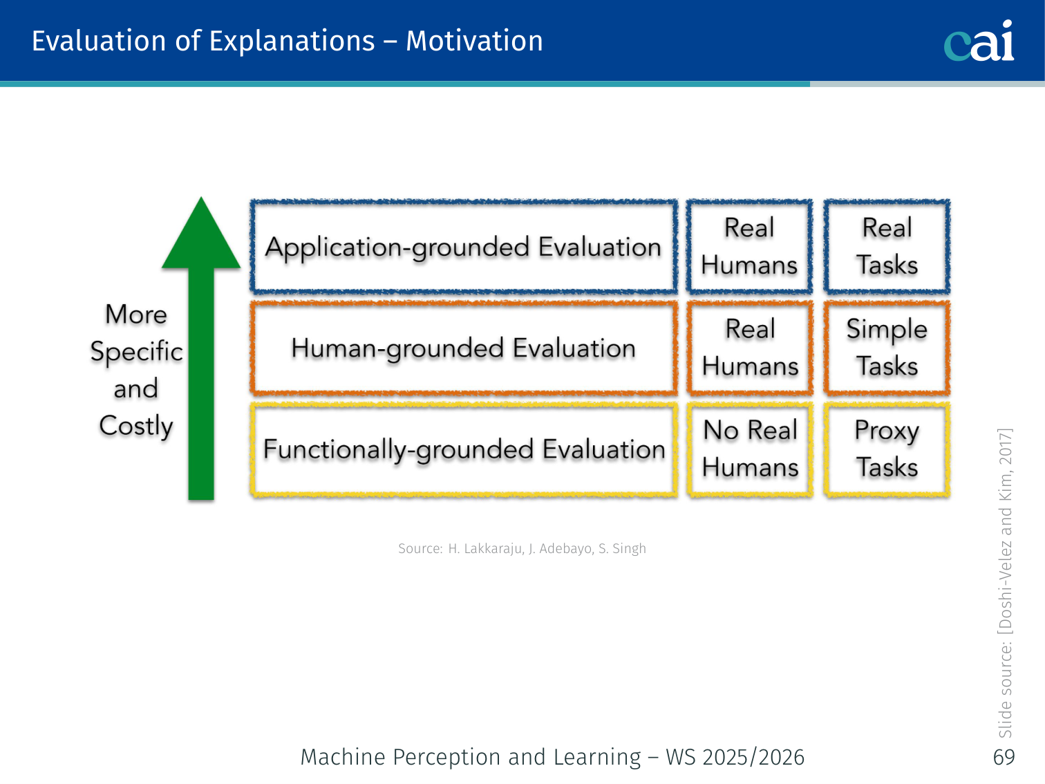
How do we know if an explanation is good? This is non-trivial — explanations exist for human consumers, so evaluation requires human studies.

Three evaluation goals [Doshi-Velez & Kim, 2017]:

1. Understand Behaviour

One goal is just to understand the model's behavior—like seeing which features it really depends on.

Tests like deletion and insertion help us measure how much each feature actually impacts the output.

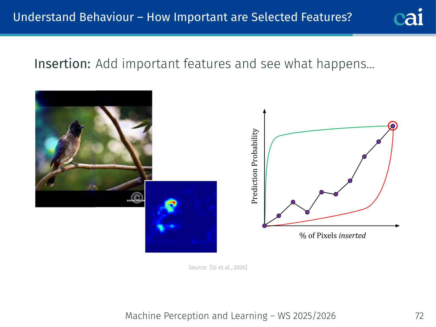
Deletion / Insertion tests [Qi et al., 2020]: Remove (or add) features in order of importance and measure the change in model prediction. A good explanation should identify features whose removal causes a sharp accuracy drop.

• Deletion: mask top-$k$ features → model performance should drop rapidly
• Insertion: start from blank and add top-$k$ features → performance should rise rapidly

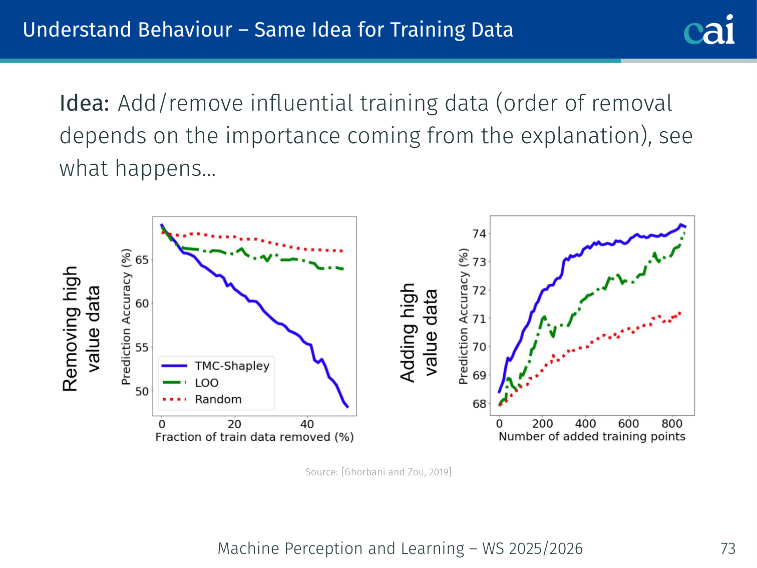
Training data influence: Add/remove influential training examples (ranked by explanation method) and observe effect on test loss [Ghorbani & Zou, 2019].

Prediction simulation: Can a user predict the model’s output on a new instance, given prior predictions and their explanations? [Ribeiro et al., 2018; Hase & Bansal, 2020; Poursabzi-Sangdeh et al., 2021]

2. Useful for Debugging

XAI is a lifesaver for debugging, helping us catch when a model is right for the wrong reasons.

Explanations can help us spot bugs or biases that might be hidden in the model's performance metrics.

• Detecting bugs: Create a deliberately buggy classifier; check if users can identify the bug given explanations [Ribeiro et al., 2016]
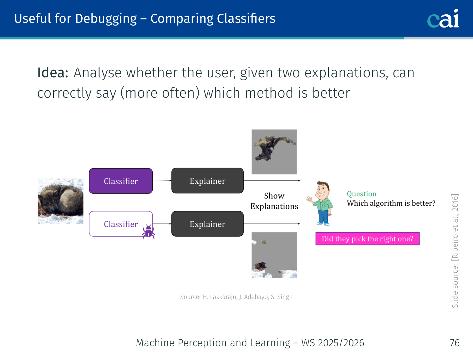
• Comparing classifiers: Given two explanations, can users correctly identify which model is better?
• Fixing features: Can users improve the model by identifying and correcting problematic features?
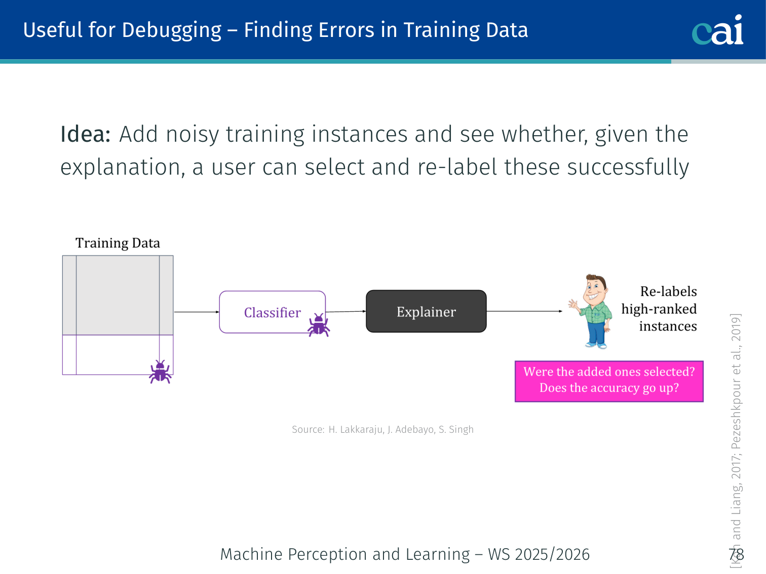
• Finding labelling errors: Add noisy (mislabelled) training instances; can users find and re-label them using the explanation? [Koh & Liang, 2017]

3. Help Make Decisions

Finally, explanations should actually help us make better decisions when collaborating with AI.

Human-AI collaboration: Are explanations useful for tasks where the algorithm alone is unreliable?

Deception detection example [Lai & Tan, 2019]: Classify fake online reviews. Humans alone perform modestly; AI alone has its own error pattern. Do explanations improve decision accuracy when humans act on AI recommendations?

---

Summary

Method	Scope	Model-Agnostic	Output
Input Gradient	Local	✗	Pixel heatmap
SmoothGrad	Local	✗	Smoothed heatmap
Integrated Gradients	Local	✗	Path-integrated attribution map
Grad-CAM	Local	✗	Spatial region map
LRP	Local	✗	Layerwise heatmap
LIME	Local	✓	Feature importances (sparse linear)
Anchors	Local	✓	Sufficient condition rule
Counterfactuals	Local	✓	“What-if” recourse
Influence functions	Local	✗	Training example attribution
Activation Maximisation	Global	✗	Neuron-activating prototype
SP-LIME	Global	✓	$k$ representative local explanations
Network Dissection	Global	✗	Neuron–concept alignment scores
SHAP / DeepSHAP	Local + Global	✓	Shapley value attributions
TCAV	Global	✗	Concept sensitivity score per layer
Probing	Global	✗	Concept decodability per layer

Key takeaways:

1. If an interpretable model achieves sufficient accuracy, prefer it over post-hoc explanations
2. No single explanation method is complete — use multiple
3. A convincing-looking explanation can still be wrong (gradient saturation, spurious correlations)
4. Always validate explanations against domain knowledge (does this make sense to an expert?)
5. Evaluation requires both automatic metrics (deletion/insertion) and human studies (debugging, simulation)

---

References

• Sundararajan, Taly, Yan (2017) — Axiomatic attribution for deep networks. ICML.

Applied Exam Focus

• Saliency Maps: Gradient-based methods (like Grad-CAM) highlight which pixels most influenced the prediction. Note: they can be noisy and misleading.
• SHAP: Based on Shapley Values from game theory. It is the only method that guarantees a fair distribution of “credit” among all input features.
• Local vs. Global: LIME provides Local explanations (for one specific image), while TCAV provides Global explanations (for a whole concept like “stripes”).

---

Previous: L12 — Diffusion | Back to MPL Index | (y) Return to Notes | (y) Return to Home