08_special_effects - Image-Space Special Effects

Back: (y-07) Deferred Shading | Next: (y-09) Semi-Global Illumination | RTG Index

Mental Model First: Effects in Image Space

Once geometry has been rasterized into a G-Buffer plus a color buffer, the rest of the frame is a 2D image-processing problem. Special effects work on those screen-sized textures, not on triangles.
A postprocessing pass is just a fullscreen fragment shader. It reads neighbouring pixels (or G-Buffer channels) and writes a new color. Cost scales with screen pixels, not scene complexity.
Two recurring primitives carry most of the chapter. A separable Gaussian filter underpins blur, bloom, depth of field. A bilateral filter (Gaussian plus a range weight on a guide channel) preserves edges and underpins depth-aware blur, denoising, and joint upsampling.
Anti-aliasing splits into sampling more (SSAA, MSAA, TAA) and filtering smarter (MLAA, TAA again). TAA is the modern gold standard because it spreads supersampling cost across frames using reprojection and history rejection.
Motion blur, lens flare, billboards, and particle systems are screen-space tricks that look expensive but cost very little. They are how engines sell realism cheaply.

1. Why Image-Space Effects

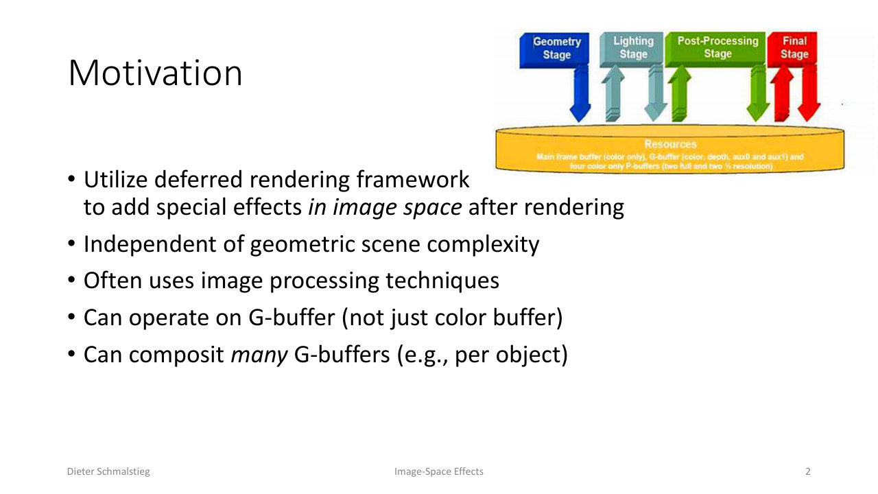
L08_Pg-02: Image-space effects extend the deferred pipeline by adding a post-processing stage that reads color and G-Buffer resources.

A deferred renderer already produces two useful intermediate products: the color buffer and the G-Buffer. Special effects piggyback on that pipeline:

they run after rasterization, as fragment shaders over fullscreen quads,
their cost is independent of scene polygon count, depending only on resolution and kernel size,
they can read any G-Buffer channel (depth, normal, motion, ID), not just the color buffer,
they can composite many partial render buffers, one per object class, to fake effects like translucency or per-object motion blur.

The pipeline shape is geometry → lighting → post-process → final, with the G-Buffer and auxiliary P-buffers as the shared resource pool.

2. Distance Fog as the Canonical Postprocess

The simplest postprocess is distance fog: blend the surface color $c_{s}$ with a fog color $c_{f}$ based on a per-pixel fog factor $f$ :

$c = f c_s + (1 - f) c_f$

When the pixel is close to the camera ( $f \approx 1$ ) it stays bright; far away ( $f \to 0$ ) it fades to fog.

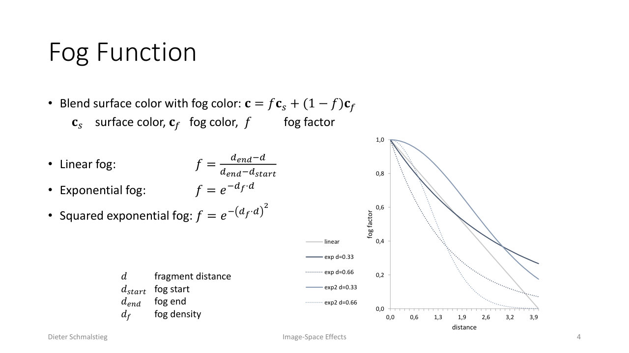
L08_Pg-04: Three fog curves - linear, exponential, and squared exponential - produce different falloff shapes.

Three standard fog curves exist:

Linear: $f = \frac{d _{e n d} - d}{d _{e n d} - d _{s t a r t}}$ , useful when fog has a clear start and end distance.
Exponential: $f = e^{- d_{f} \cdot d}$ , physically motivated for uniformly absorbing media.
Squared exponential: $f = e^{- (d_{f} \cdot d)^{2}}$ , a softer near-camera transition with a sharper far-distance falloff.

Implementation is trivial: read the view-space position from the G-Buffer (or reconstruct from depth), compute $d = ∥ p_{c am} - p ∥$ , evaluate the fog curve, and blend.

💡 Intuition

Fog is the first non-trivial “shader runs once per pixel” effect because it depends only on per-pixel data and one constant. Everything else in this lecture follows the same template, just with bigger kernels and more inputs.

3. Image Processing in a Pixel Shader: Gaussian Blur

Image processing means computing some derivative function of a pixel’s neighbourhood. The workhorse is the Gaussian blur, which weighs samples by a 2D Gaussian kernel.

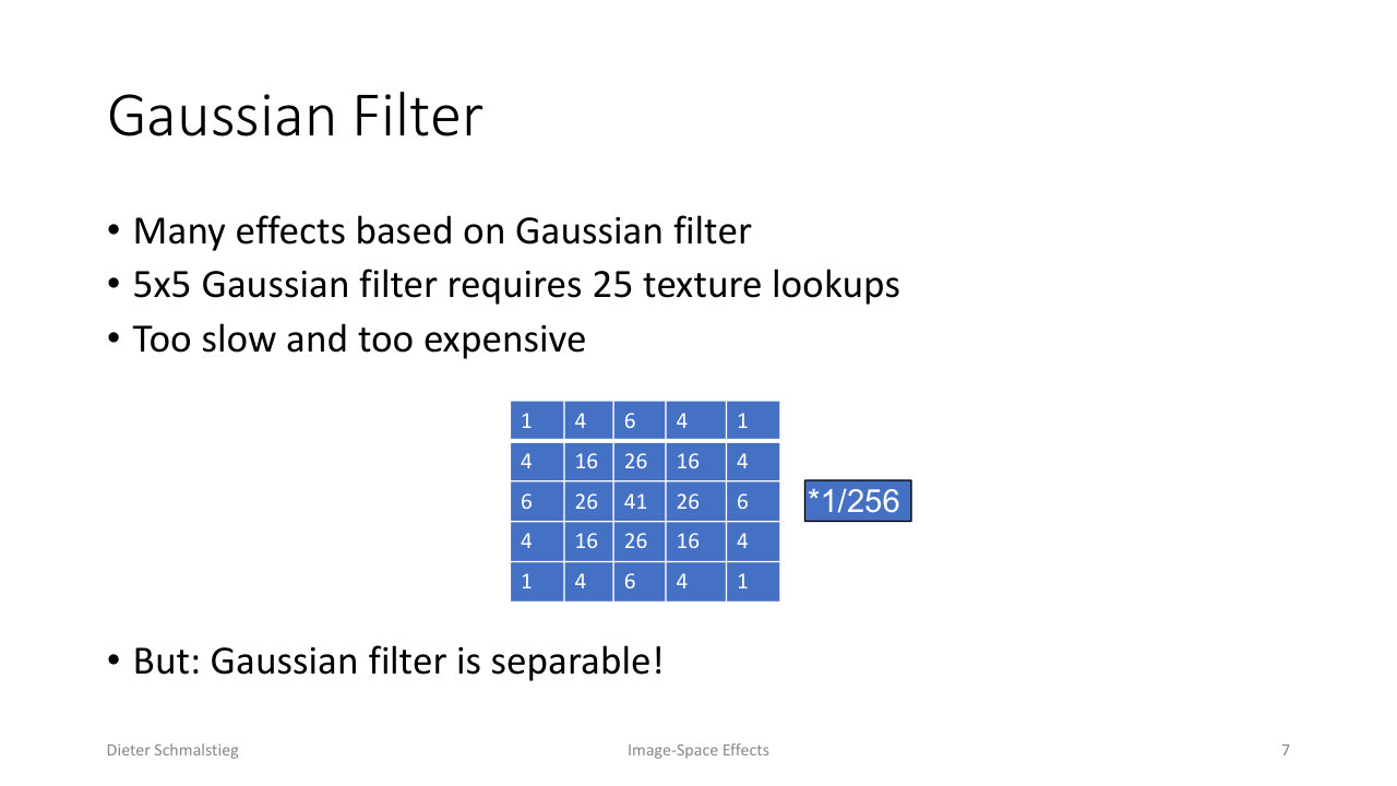
L08_Pg-07: A 5x5 Gaussian kernel costs 25 texture lookups per pixel before normalization by 1/256.

A naive 5x5 Gaussian kernel needs 25 texture lookups per output pixel, which is far too expensive at high resolution. The standard rescue is separability.

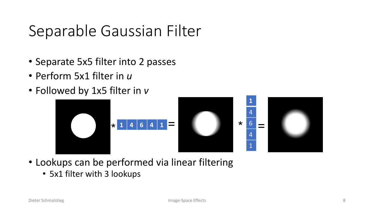
L08_Pg-08: A 2D Gaussian is the outer product of two 1D Gaussians, so a 5x5 filter becomes 5+5 = 10 lookups in two passes.

A Gaussian kernel factorizes as the outer product of two 1D kernels, so a 5x5 filter is two passes of a 5x1 filter (one horizontal, one vertical), reducing 25 lookups to 10. Hardware bilinear filtering can collapse pairs of adjacent samples, so a 5x1 pass needs only three lookups in practice.

The actual shader is a one-pass loop over num_samples along a direction vector that is (1,0) in the horizontal pass and (0,1) in the vertical pass, selected by a preprocessor flag like #ifdef BLUR_Y.

🧠 Deep Dive: Why Separability Matters

A $k \times k$ kernel costs $k^{2}$ texture taps per pixel. Two separable passes cost $2 k$ . At $k = 5$ that is 25 vs 10. At $k = 31$ (a strong blur for bloom or DoF) it is 961 vs 62, an order-of-magnitude saving. This is why every blur in a real-time engine is implemented as two 1D passes and why kernels that are not separable (true bilateral, true anisotropic) need extra tricks to stay fast.

4. Bloom

Bright areas of a real image bleed light into their neighbourhood because of glare in the optics and the eye. The graphics version is bloom: blur the bright parts and add the blurred image back to the original.

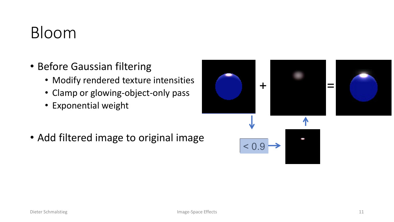
L08_Pg-11: Bloom isolates bright pixels with a threshold, blurs them, then adds the blurred glow back on top of the original.

The full bloom recipe:

Threshold the rendered color buffer to keep only intensities above some cutoff (or render only glowing objects into a separate pass).
Blur that bright-only image with a separable Gaussian, usually after downsampling 2x or 4x to widen the effective kernel cheaply.
Add the blurred result back on top of the original color buffer.

Practical refinements:

Downsample then blur because a fixed-size kernel covers more screen area at lower resolution, but sharp highlights soften.
Combine multiple downsample levels with different blur radii to give artists control over both halo width and core brightness.
A star effect is bloom with the horizontal and vertical passes added separately instead of combined.
Bloom hides aliasing artifacts, which is why it became overused. Use it sparingly, mostly on sun and sky, on shiny materials, or only on the specular term. Heavy bloom smudges out a scene into a “fairytale look” with no sharp contrast.

5. Depth of Field

Cameras and eyes can only focus on one depth at a time. Objects at the focal plane appear sharp; everything else blurs by an amount proportional to its distance from the focal plane.

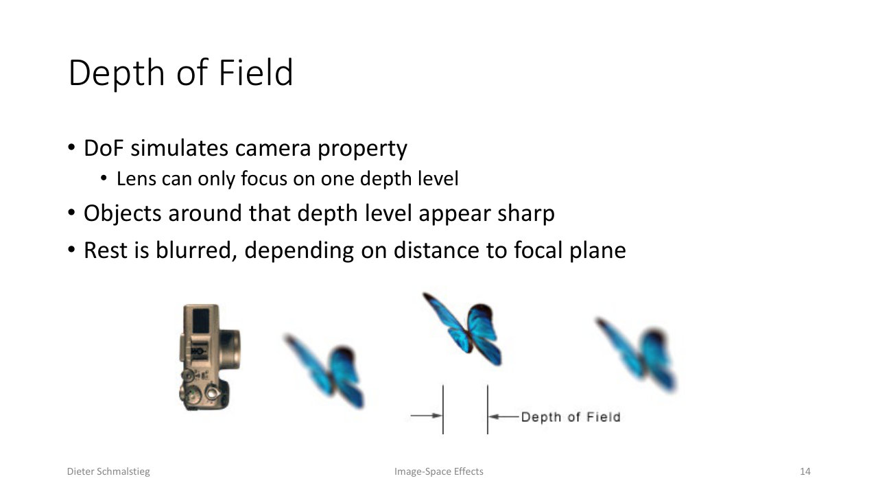
L08_Pg-14: DoF simulates a real lens, where objects far from the focal plane progressively blur.

Image-space DoF turns this into a postprocess:

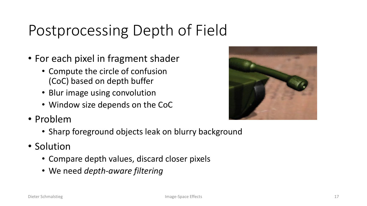
L08_Pg-17: Per pixel, the circle of confusion comes from depth, then a convolution blurs by that radius - but naive filtering leaks foreground into background.

For each pixel:

Read its depth from the G-Buffer.
Compute the circle of confusion (CoC) radius from how far that depth is from the focal plane.
Blur the image with a convolution whose window size matches the CoC.

The problem: a naive blur lets sharp foreground objects leak onto their blurry background, because the blur kernel happily samples across the silhouette. The fix is depth-aware filtering: discard sample contributions when their depth differs strongly from the centre pixel’s depth.

6. Bilateral and Joint Bilateral Filters

A Gaussian filter only weighs samples by spatial distance, so it always blurs. A bilateral filter also weighs samples by the difference between their colors and the centre pixel’s color (range weight). Samples whose color differs strongly are downweighted, so the filter preserves color discontinuities while still smoothing within regions.

The joint bilateral filter decouples the range weight from the image being filtered. Instead, range weights come from a separate guide channel - typically the depth buffer or a normal buffer.

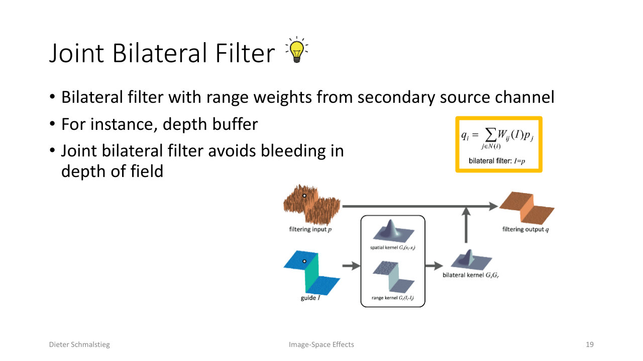
L08_Pg-19: A joint bilateral filter weights samples by spatial distance and by similarity in a guide channel (e.g. depth), giving edge-preserving blur.

This is exactly the tool the depth-of-field problem needs: the guide channel is depth, so the blur stays confined to surfaces that share the centre pixel’s depth and stops bleeding across silhouettes.

💡 Intuition

A Gaussian asks “how close is this sample in screen space?” A bilateral filter also asks “how similar is its color?” A joint bilateral filter substitutes “how similar is its depth (or normal, or object ID)?” - using whichever auxiliary channel best identifies the boundary you want to preserve.

7. Edge Detection in Image Space

Postprocesses can also detect edges by running a derivative filter on a screen-sized buffer.

A first-order differential (Sobel) on the depth buffer picks out depth discontinuities, which correspond to object silhouettes. This is called the profile edge.
A second-order differential (Laplacian) picks out depth inflection points: ridges and creases inside a surface. This is the internal edge.

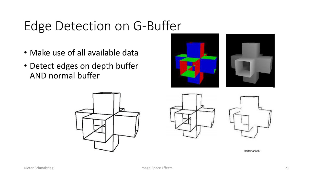
L08_Pg-21: Running edge detection on both the depth buffer and the normal buffer catches silhouettes the depth alone misses.

Running edges on depth alone misses silhouettes where two surfaces meet at almost the same depth (e.g. two faces of a folded sheet of paper). Adding edge detection on the normal buffer rescues those cases.

Pros and cons of image-space edges:

Pro: cost is independent of polygon count.
Con: cost depends on screen resolution, and the same scene gives different edges when zoomed in or out.
Con: z-fighting and small depth errors produce noisy edges, especially on near-coplanar surfaces.

This is the basis of cartoon outlines and toon shaders, and the same trick is used by morphological anti-aliasing (MLAA) later in the lecture.

8. Non-Photorealistic Rendering with G-Buffers

The G-Buffer is also the right input for many NPR effects. Hatching, for example, applies brush strokes that follow the surface’s $(u, v)$ coordinates so the strokes wrap with the geometry.

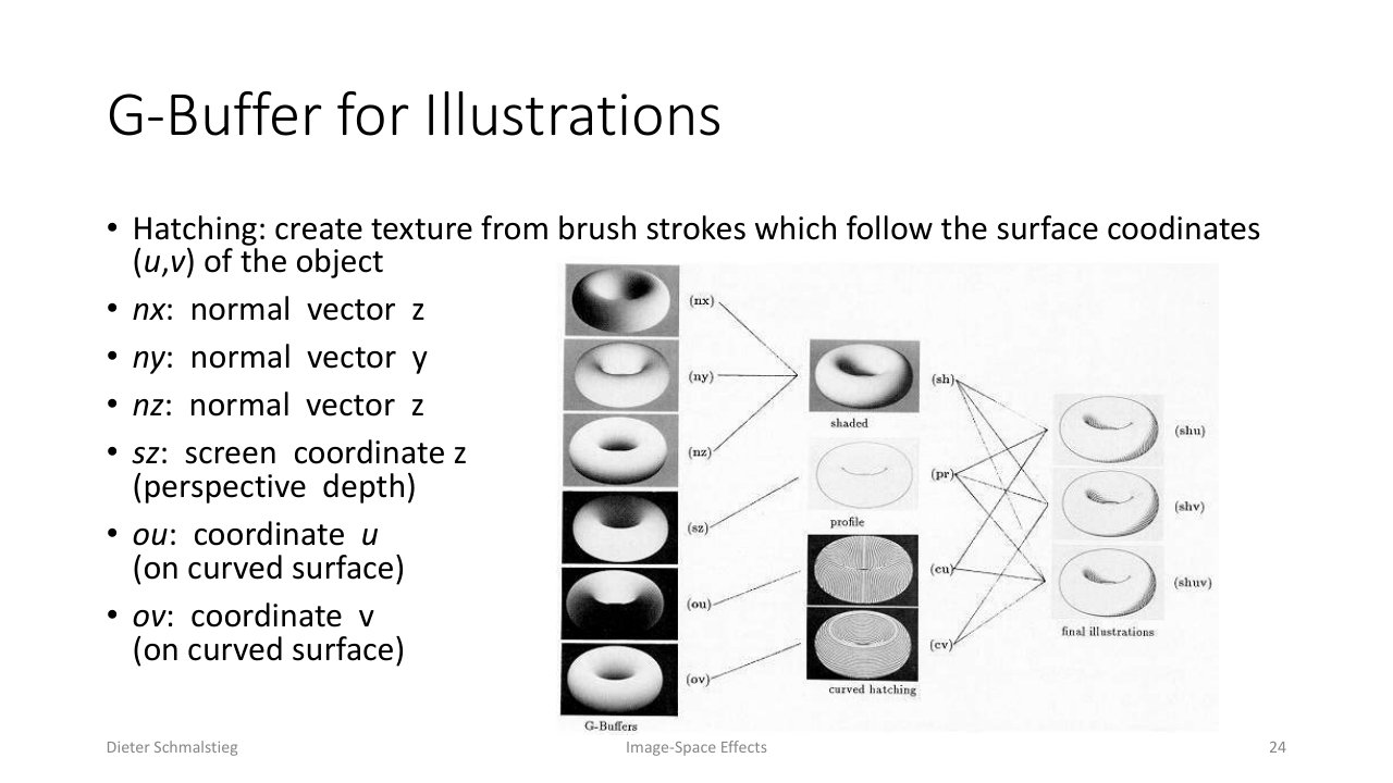
L08_Pg-24: A G-Buffer of normals, screen depth, and surface (u, v) coordinates drives hatching that follows the surface, profile, and curvature.

The trick is to add extra G-Buffer channels for whatever the NPR algorithm needs - in this example, the three normal components, perspective depth, and the surface $u$ and $v$ - and compose the final illustration from filters over those channels.

9. Upsampling and DLSS

Rendering at lower resolution and upsampling is a cheap way to recover frame rate. Naive bilinear upsampling kills high-frequency detail; joint bilateral upsampling (color as primary channel, depth or ID buffer as guide) preserves edges much better.

On PS4 Pro, for instance, the GPU has 4x more pixels to fill but only 2x more cores, so the driver renders color at quarter resolution, an edge buffer at full resolution, and joint-bilateral upsamples the color using the edge buffer as guide - all transparent to the game engine.

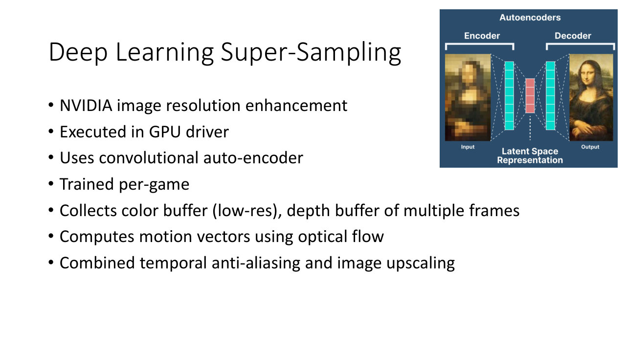
L08_Pg-27: DLSS is a per-game convolutional auto-encoder that combines temporal anti-aliasing with image upscaling, executed entirely in the GPU driver.

Deep Learning Super-Sampling (NVIDIA DLSS) is the modern evolution: a convolutional auto-encoder, trained per game, takes a low-resolution color buffer plus depth and motion vectors from multiple frames and outputs a high-resolution, temporally stable image. It runs in the GPU driver, combining temporal anti-aliasing and upscaling into a single learned pass.

10. Anti-Aliasing in Real-Time Graphics

Anti-aliasing has two flavors: sample more during rasterization (SSAA, MSAA, TAA) and filter smarter afterwards (MLAA, TAA).

Supersampled Anti-Aliasing (SSAA)

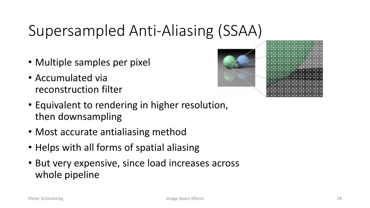
L08_Pg-29: SSAA takes many samples per pixel, then accumulates them via a reconstruction filter - equivalent to rendering at higher resolution and downsampling.

SSAA allocates every screen-sized texture and buffer at $N \times$ the target resolution, renders normally at that higher resolution, then downsamples to the target with a box, Lanczos, or Gaussian filter. It is the most accurate AA method and helps with every kind of spatial aliasing (geometry, textures, shading) - but every pipeline stage runs $N$ times as much work.

Multisample Anti-Aliasing (MSAA)

Most visible aliasing is “jaggies” at triangle edges. MSAA places multiple subsamples per pixel for coverage and depth tests, but runs the fragment shader only once per pixel. The output color is then blended based on how many of the subsamples were covered. Hardware support is built into every graphics API.

MSAA is cheaper than SSAA because shading runs once per pixel, but it only fixes edge aliasing - not texture or shading aliasing - and it does not compose with deferred rendering, because shading happens after rasterization on a single per-pixel G-Buffer.

Morphological Anti-Aliasing (MLAA)

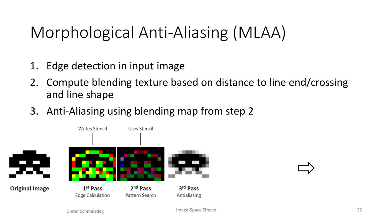
L08_Pg-32: MLAA is a three-pass post-process: detect edges, compute a blending texture from line shapes, then blend along edges.

MLAA is a post-process applied after the frame is rendered:

Edge detection on the input image.
Compute a blending texture based on the distance from each pixel to a detected line end or crossing, and the shape of that line.
Blend the image along the detected edges using the blending map.

It is cheap even on weak hardware and is the preferred AA for deferred rendering engines, but it blurs only along detected edges, can soften fine details like text, and is not temporally stable, so edges flicker frame to frame.

Comparison

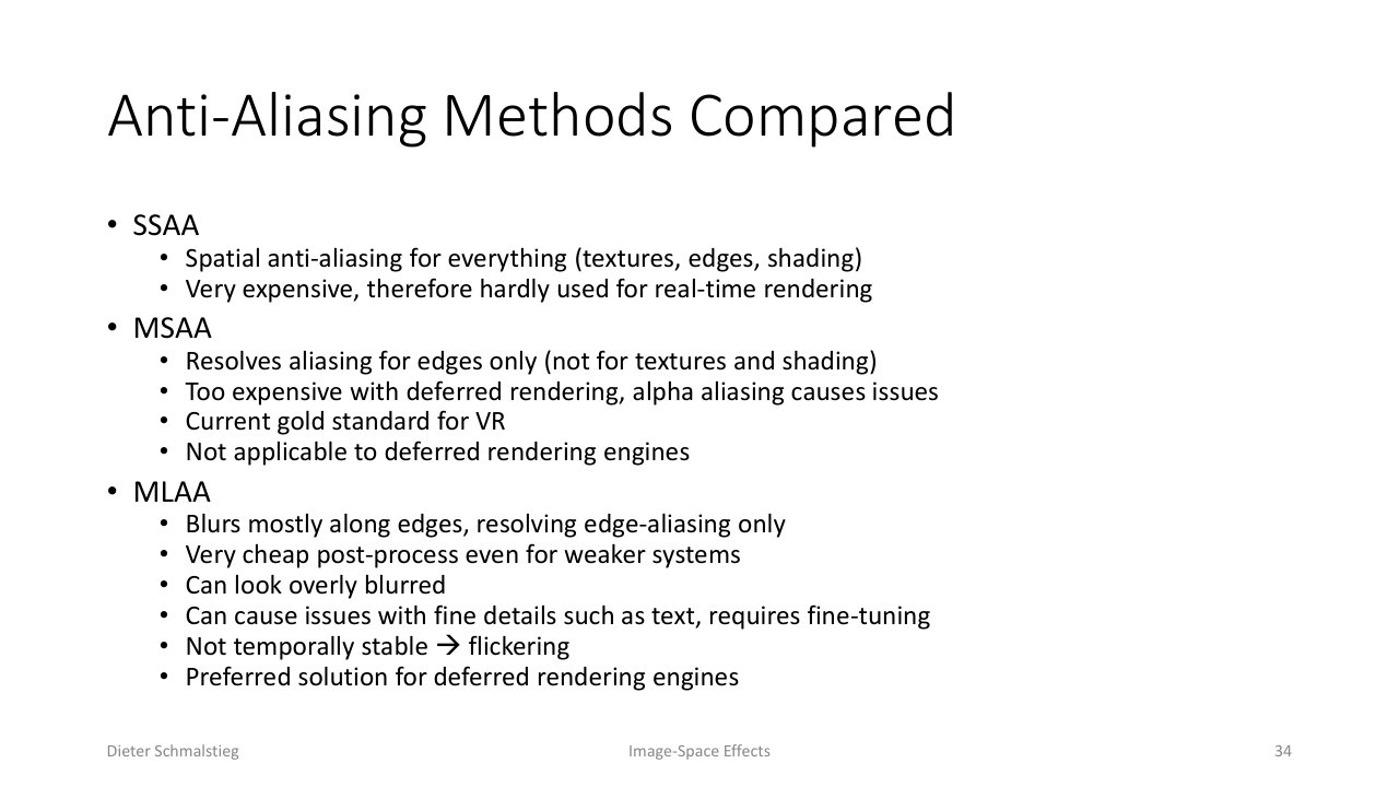
L08_Pg-34: Summary - SSAA is universal but expensive, MSAA fixes only edges and breaks with deferred, MLAA is cheap but flickers.

SSAA: spatial AA for everything; too expensive for real-time.
MSAA: fixes edges only; the gold standard for VR but not applicable to deferred engines.
MLAA: cheap blur along detected edges; preferred for deferred engines but flickers and softens fine detail.

11. Temporal Anti-Aliasing (TAA)

The modern dominant AA approach is TAA: spread supersampling across time by combining one new sample per pixel per frame with stored samples from previous frames. It works for both geometric and shading aliasing, scales with any rendering architecture, and is the current gold standard for game engines.

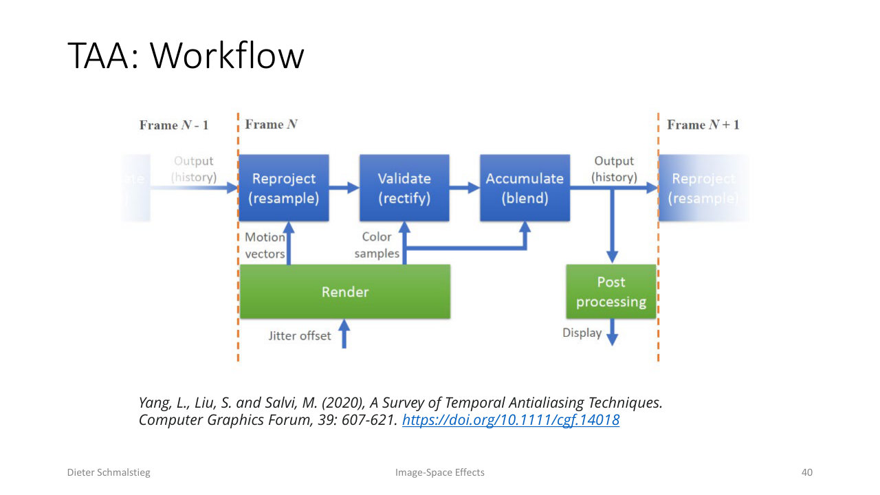
L08_Pg-40: TAA reprojects the previous output (history), validates and rectifies it against current samples, then accumulates the blend, ready to feed the next frame.

The TAA pipeline per frame is reproject → validate → accumulate, taking the previous output (history), motion vectors, and current color samples as inputs and producing both the output image and the next frame’s history.

Jittering

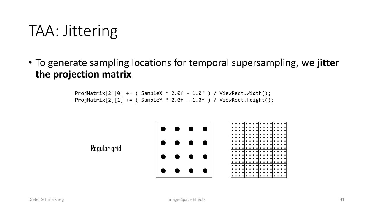
L08_Pg-41: Jittering offsets the projection matrix by sub-pixel fractions each frame, so each frame samples a different point inside the pixel.

To get supersampling for free, TAA jitters the projection matrix every frame by a sub-pixel offset, so the same pixel is sampled at different sub-pixel positions across successive frames. Code-wise it is two lines:

ProjMatrix[2][0] += (SampleX * 2.0f - 1.0f) / ViewRect.Width();
ProjMatrix[2][1] += (SampleY * 2.0f - 1.0f) / ViewRect.Height();

Each frame’s subsequence of jitter offsets should still be evenly distributed over the pixel; Halton(2,3) is the standard low-discrepancy sequence (used by Unreal Engine 4) because every prefix of the sequence stays well distributed.

History Buffering

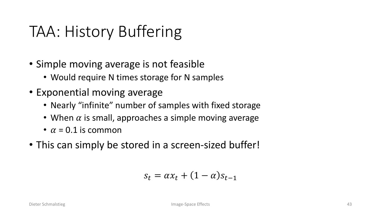
L08_Pg-43: TAA stores history as an exponential moving average, $s_t = \alpha x_t + (1 - \alpha) s_{t-1}$, giving infinite samples in fixed storage.

A simple moving average of the last $N$ frames would need $N$ times the storage. The trick is an exponential moving average:

$s * t = α x_{t} + (1 - α) s * t - 1$

with $α \approx 0.1$ . It approximates a long-window average using only one screen-sized history buffer, and as $α \to 0$ the result approaches a true moving average.

Reconstruction inside a pixel is then a weighted sum of the contributing subpixel samples. UE4 uses a Gaussian fit to a Blackman-Harris 3.3 window, precomputed once and passed as shader uniforms.

Reprojection for Dynamic Scenes

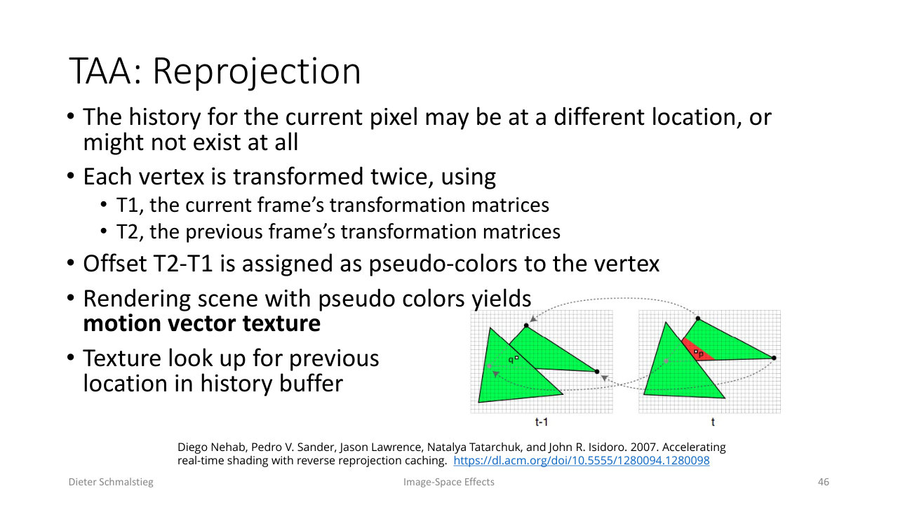
L08_Pg-46: Each vertex is transformed by both the previous and current frame's matrices; their difference is rendered as a per-pixel motion vector texture.

When the camera moves or objects animate, the history sample for a pixel is no longer at the same screen position. Reprojection computes per-pixel motion vectors and uses them to look up the right history pixel.

The motion vector is built by transforming each vertex twice: by the previous frame’s matrices $T_{1}$ and the current frame’s $T_{2}$ . The difference $T_{2} - T_{1}$ becomes a pseudo-color attribute and the scene is rendered with that pseudo-color to produce a motion-vector texture.

History Rejection and Rectification

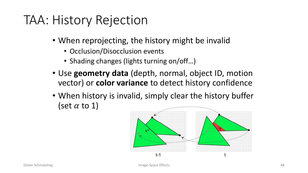
L08_Pg-48: Reprojected history is invalid at occlusion or disocclusion events, or when shading changes - use geometry data (depth, normal, ID, motion) or color variance to detect and clear it.

Reprojected history is sometimes wrong:

Occlusion or disocclusion: a pixel is showing a different surface than last frame.
Shading changes: a light turned on or off, or a material switched.

If history is invalid, simply clear it (set $α = 1$ , so the next frame is the new sample alone). Detection uses geometry data (depth, normal, object ID, motion vector mismatch) or color variance in the neighbourhood.

A softer alternative is history rectification: instead of throwing the history away, clip it into the AABB or convex hull of the current pixel’s $3 \times 3$ neighbourhood in color space. The clipped color is then a plausible neighbour of the new samples and can still be blended in.

Without all this care, TAA produces ghosting: faint trails behind moving objects where the history persists where it should not.

12. Motion Blur

Real cameras and human eyes blur fast-moving objects, because exposure or persistence integrates motion over a short time window. Adding motion blur to a real-time render is both visually flattering and a way to hide low frame rate.

Discrete vs Continuous

The simplest discrete method is to draw the object at several past positions with decreasing opacity. It needs multiple draws per object. Image-space motion blur renders the object to a buffer once and composites the buffer at past positions, which is cheaper.

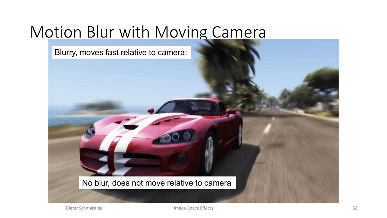
L08_Pg-52: Motion blur is relative to the camera - palm trees streak past a moving car while the car itself stays sharp.

Real motion blur is relative to the camera, not the world. In a chase shot, the car is stationary in screen space while the background streaks past.

Continuous Motion Blur via a Velocity Buffer

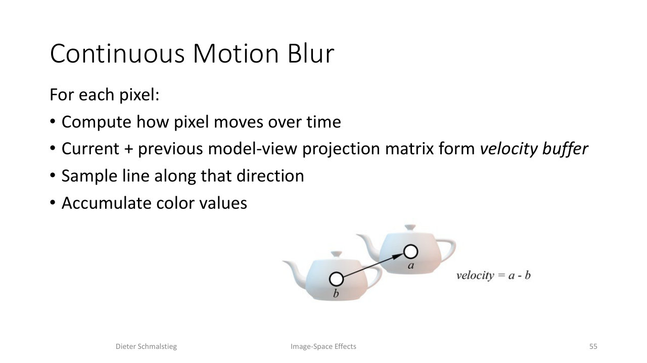
L08_Pg-55: Per-pixel velocity = current position - previous position; sample along that direction in the color buffer and accumulate.

The standard continuous method is the same idea as TAA reprojection:

Compute a per-pixel velocity buffer from the current and previous frame’s model-view-projection matrices.
For each pixel, sample the color buffer along the velocity direction.
Accumulate the samples.

The result is a blur whose direction and length come naturally from per-pixel screen-space motion.

Artifacts

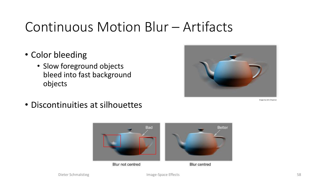
L08_Pg-58: Discontinuities at silhouettes and color bleeding from slow foreground into fast background; centring the blur helps.

Two classic motion-blur artifacts:

Color bleeding: a slow foreground object leaks into a fast-moving background because the blur kernel samples across the silhouette.
Silhouette discontinuities: the blur is asymmetric around the object boundary; centring the blur around the pixel position instead of trailing behind it looks better.

13. Image Compositing: Lens Flare

Lens flare is a camera defect (light scattering inside the lens system) that photographers usually try to avoid, but it looks cinematic in games. The effect is always rendered on top of the scene, since it happens inside the lens.

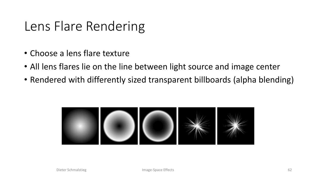
L08_Pg-62: Lens flare is rendered as alpha-blended billboards strung along the line between the light source and the image centre.

Recipe:

Choose a set of lens-flare textures (haloes, rings, stars).
Place them on the line between the light source’s screen position and the image centre, at different distances along that line.
Render each as a transparent billboard with alpha blending.

The line geometry makes the flare slide across the screen as the camera turns, which is what sells the illusion. As with bloom: do not overdo it.

14. Billboards

Billboards (also called impostors or sprites) are textured rectangles that always face the camera or align with a fixed axis. They are simple - two triangles plus a texture - and trivially cheap, so they are the go-to representation for distant or small objects.

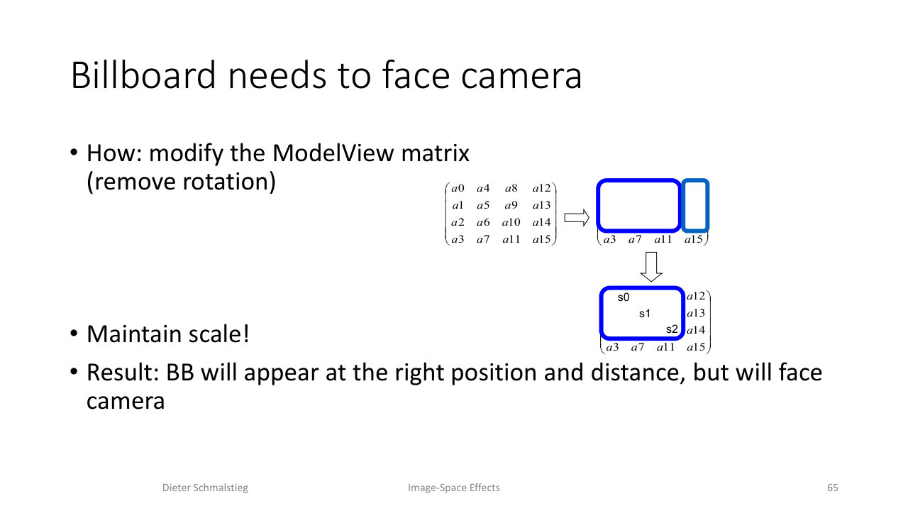
L08_Pg-65: To make a billboard face the camera, replace the rotation portion of the ModelView matrix with identity, keeping translation and scale.

To make a billboard always face the camera, modify the ModelView matrix: zero out the rotation portion (replace the top-left $3 \times 3$ with identity scaled by $(s_{0}, s_{1}, s_{2})$ ) while keeping the translation column and the scale, so the billboard ends up at the right position and distance but facing the camera.

A billboard cloud is many billboards with varied size and orientation, generated procedurally from a 3D model or rule set, used for trees and foliage and animated by simple physics.

15. Particle Systems

Particle systems model things that change over time: rain, snow, fire, smoke, explosions, sparks, sprays. They are typically large numbers of small objects rendered as billboards, with shared update logic.

The 1982 Genesis sequence in Star Trek II is the canonical historical example.

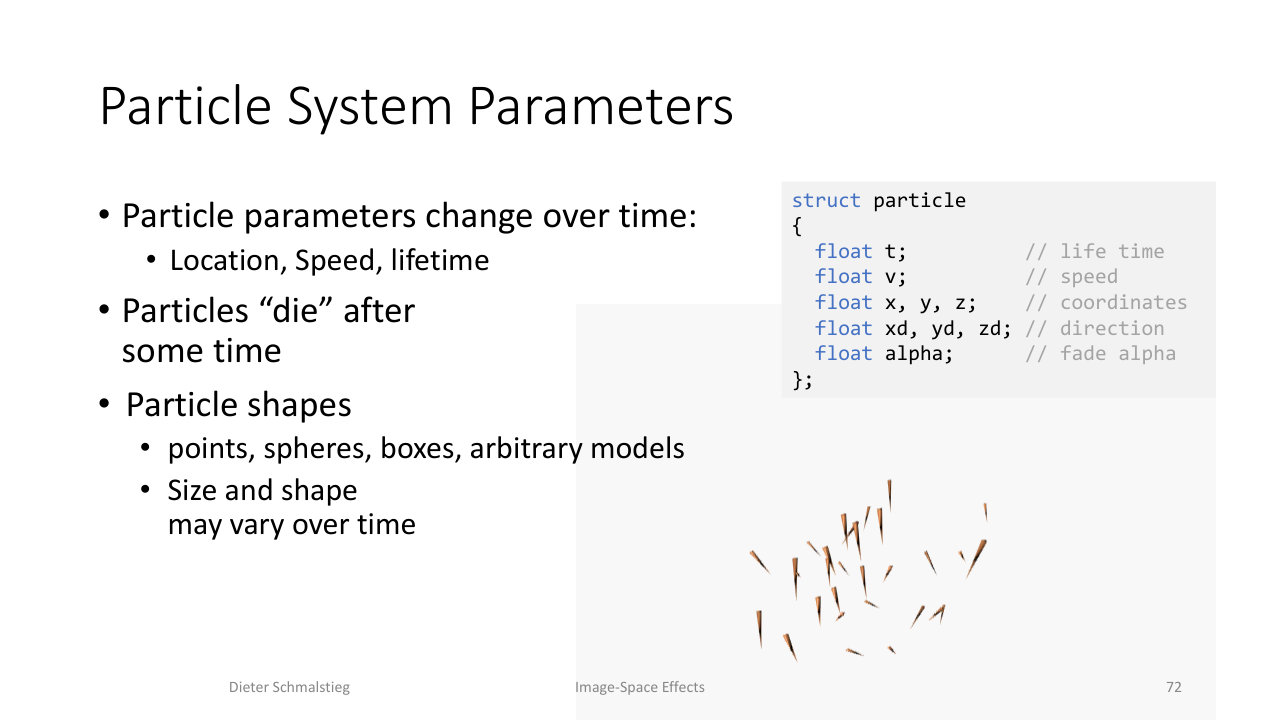
L08_Pg-72: A minimal particle struct: lifetime, speed, position, direction, alpha - varied over time by a shared update rule.

A particle struct stores at minimum lifetime, speed, position, direction, and an alpha. The system handles:

Initialization (spawn from an emitter shape, with random jitter on parameters),
Update (advance position by velocity, apply external forces such as gravity or collision),
Randomness (using cheap PRNGs to give each particle a unique trajectory),
Rendering (typically as billboards, sometimes with simple shapes such as spheres or boxes).

Particles die after their lifetime expires. They can interact with each other for more entropic effects like liquid sprays. The engineering priorities are fast physics and collision, low memory per particle, and fast rendering - not physical correctness.

State-less particles derive their position purely from time and initial conditions (useful for GPU implementation). State-full particles carry mutable per-frame state, allowing collisions and other dependencies on the world.

Applied Exam Focus

Postprocess template: read color and/or G-Buffer channels in a fullscreen fragment shader and write a modified color. Independent of polygon count, scales with screen pixels.
Distance fog: blend $c = f c_{s} + (1 - f) c_{f}$ with linear / exponential / squared-exponential curves.
Separable Gaussian: a $k \times k$ Gaussian blur becomes two 1D passes, dropping cost from $k^{2}$ to $2 k$ texture taps per pixel.
Bloom: threshold bright pixels → blur (often after downsampling) → add back; hides aliasing but smudges the scene if overdone.
Depth of field: per-pixel circle of confusion from depth, blur with a kernel of that radius, use depth-aware (joint bilateral) filtering to stop foreground leaking onto background.
Bilateral / joint bilateral filter: Gaussian plus a range weight on color (bilateral) or a guide channel like depth (joint bilateral). Preserves edges.
Image-space edge detection: Sobel on depth gives profile edges, Laplacian gives internal edges; depth alone misses near-coplanar silhouettes, so include the normal buffer.
Joint bilateral upsampling: render color at low resolution, an edge or depth buffer at full resolution, upsample color using the edge buffer as guide (PS4 Pro driver). DLSS does the same idea with a per-game neural net.
Anti-aliasing:
- SSAA: render at $N \times$ resolution and downsample - fixes everything but very expensive.
- MSAA: more depth/coverage samples per pixel, fragment shader runs once - fixes only edges, breaks with deferred.
- MLAA: post-process edge detection plus blend, cheap but flickers and softens fine detail.
- TAA: jitter projection matrix per frame with Halton(2,3), accumulate history with exponential moving average ( $α \approx 0.1$ ), reproject using per-pixel motion vectors, reject or rectify invalid history (occlusion, shading change, neighbourhood-AABB clip).
Motion blur: continuous version builds a per-pixel velocity buffer from current and previous MVP matrices, samples the color buffer along that direction, accumulates. Centring the blur reduces silhouette artifacts.
Lens flare: alpha-blended billboards along the line from light source to image centre, rendered on top of everything.
Billboards and particle systems: face-camera quads with two triangles each; particle systems share an update rule across many short-lived billboards. Cheap, used heavily for foliage, smoke, fire, sparks.

Self-Check

Why is a separable Gaussian filter dramatically faster than the equivalent 2D Gaussian, and what is the cost difference for a 5x5 kernel?

Answer

A 2D Gaussian factorizes as the outer product of two 1D Gaussians, so the same blur can be computed in two passes - once horizontally and once vertically. A direct $k \times k$ kernel costs $k^{2}$ texture taps per pixel; two separable 1D passes cost $2 k$ . For $k = 5$ that is 25 vs 10 taps; hardware bilinear filtering can collapse a 5x1 pass to three taps in practice.

Why does naive depth-of-field bleed sharp foreground objects onto blurry backgrounds, and what filter fixes it?

Answer

A naive blur averages neighbouring pixels regardless of depth, so kernel samples cross the silhouette and pull foreground color into the background. The fix is a depth-aware (joint bilateral) filter: weight samples not only by spatial distance but also by similarity to the centre pixel’s depth in the G-Buffer, so samples on the other side of a depth discontinuity are downweighted to zero.

Why is MSAA not a good fit for deferred rendering, and what AA does the lecture present as the modern gold standard?

Answer

MSAA places extra coverage samples per pixel during rasterization but runs the fragment shader once per pixel. In a deferred renderer, shading happens after rasterization on a single per-pixel G-Buffer, so the extra coverage samples can no longer cheaply share shading. The modern gold standard is TAA: it jitters the projection matrix each frame, accumulates samples in a history buffer (exponential moving average), reprojects with motion vectors, and rejects or rectifies invalid history.

What is the role of the motion vector texture in TAA, and how is it generated?

Answer

The motion vector texture tells TAA where each current pixel was last frame, so its history sample can be fetched from the right screen position even when the camera or objects moved. It is generated by transforming each vertex twice - once with the current frame’s MVP matrix and once with the previous frame’s MVP matrix - then writing the per-vertex offset as a pseudo-color into the framebuffer, which the rasterizer interpolates per pixel.

How is continuous motion blur implemented in image space?

Answer

Per pixel, compute a velocity vector from the current and previous frame’s MVP matrices, store it in a velocity buffer, then sample the color buffer along that velocity direction and accumulate the samples. The direction and length of the blur come naturally from per-pixel screen-space motion, so fast objects streak more than slow ones and a moving camera blurs the background relative to whatever is stationary in screen space.

Why are lens flares always composited on top of the scene rather than depth-tested, and how are their positions chosen?

Answer

Lens flare physically happens inside the camera’s lens system, after the light has already reached the optics, so it should appear in front of every rendered surface. Its component textures (haloes, rings, stars) are placed along the screen-space line between the light source’s projected position and the image centre, at various distances along that line, and rendered as alpha-blended billboards on top of the scene.

Compare SSAA, MSAA, and MLAA in terms of what they fix and what they cost.

Answer

SSAA renders the entire frame at $N \times$ resolution and downsamples - the most accurate, fixing geometry, texture, and shading aliasing - but the entire pipeline runs $N$ times as much work, so it is too expensive for real-time. MSAA places multiple coverage/depth subsamples per pixel but runs the fragment shader only once, fixing edge aliasing cheaply; it does not address texture or shading aliasing, and breaks with deferred shading because shading happens after G-Buffer rasterization on per-pixel data. MLAA is a post-process: detect edges in the rendered image, then blend along those edges based on the detected line shape. It is cheap even on weak hardware and works with deferred, but blurs only at detected edges, softens fine details like text, and is not temporally stable, so edges flicker between frames.

Why does TAA need both jittering and reprojection, and what is the role of history rectification?

Answer

Jittering offsets the projection matrix every frame by a sub-pixel amount (commonly Halton(2,3)), so the same pixel samples a different sub-pixel position each frame, giving stochastic supersampling. Reprojection uses per-pixel motion vectors to locate the previous frame’s sample for the current pixel, since the camera or objects may have moved. Without reprojection, moving content would never accumulate a coherent history. History rectification addresses cases where the reprojected history is wrong (occlusion, disocclusion, shading change) by clipping the history colour to the AABB or convex hull of the current pixel’s $3 \times 3$ neighbourhood in colour space - keeping a plausible neighbour rather than throwing the history away entirely. Without rectification, TAA produces visible ghosting trails behind moving objects.

Back: (y-07) Deferred Shading | Next: (y-09) Semi-Global Illumination | RTG Index

Yusuf's Thoughts

Explorer

08_special_effects - Image-Space Special Effects

Mental Model First: Effects in Image Space

1. Why Image-Space Effects

2. Distance Fog as the Canonical Postprocess

💡 Intuition

3. Image Processing in a Pixel Shader: Gaussian Blur

🧠 Deep Dive: Why Separability Matters

4. Bloom

5. Depth of Field

6. Bilateral and Joint Bilateral Filters

💡 Intuition

7. Edge Detection in Image Space

8. Non-Photorealistic Rendering with G-Buffers

9. Upsampling and DLSS

10. Anti-Aliasing in Real-Time Graphics

Supersampled Anti-Aliasing (SSAA)

Multisample Anti-Aliasing (MSAA)

Morphological Anti-Aliasing (MLAA)

Comparison

11. Temporal Anti-Aliasing (TAA)

Jittering

History Buffering

Reprojection for Dynamic Scenes

History Rejection and Rectification

12. Motion Blur

Discrete vs Continuous

Continuous Motion Blur via a Velocity Buffer

Artifacts

13. Image Compositing: Lens Flare

14. Billboards

15. Particle Systems

Applied Exam Focus

Self-Check

Graph View

Backlinks