09_semi_global_illumination - Semi-Global Illumination

Back: (y-08) Image-Space Special Effects | RTG Index | Next: (y-10) Real-Time Global Illumination

Mental Model First: Cheap Tricks for Light That Travels

• Full global illumination tracks every light bounce through the scene; in real time, that is unaffordable. Semi-global illumination computes local lighting everywhere and global lighting only selectively - only for visually important effects, only for surfaces that benefit from it.
• The big global effects are reflections, refractions, transparency, shadows, and ambient occlusion. Each gets its own specialized two-pass technique: first compute the global information into an auxiliary buffer (depth map, stencil, history list, light’s-eye view), then use that buffer when shading the camera view.
• Reflections come in three flavors. Planar reflections via stencil masking are exact but only on flat surfaces. Shader-based reflections add fading and refraction on top. Screen-space reflections ray-march the depth buffer and are cheap but limited to whatever is on screen.
• Transparency is order-dependent. Correct alpha blending requires back-to-front order. The three solutions - explicit sort, depth peeling, per-pixel linked lists - trade memory bandwidth against geometry overhead.
• Shadow techniques split into two families. Shadow mapping renders depth from the light’s point of view, then compares per-pixel; fast and general but aliases. Shadow volumes extrude silhouette geometry and count ray crossings in a stencil buffer; exact but expensive.
• Ambient occlusion fakes the global contribution of bounced light by darkening surfaces that are visually crowded. The screen-space variant (SSAO) samples the depth buffer; SSDO adds direction and a single bounce for color bleeding.

---

1. The Semi-Global Recipe

Full global illumination - tracking every light bounce through the scene - is too expensive for real-time rendering. The practical compromise is:

• compute local lighting everywhere (Phong, Cook-Torrance, deferred shading from L08),
• compute global light transport selectively: only certain transport types (reflections, refractions, shadows, AO, transparency), only for objects where it matters visually,
• everything is a two-pass technique: first build an auxiliary buffer that captures the global information, then read it during the normal render.

The recurring pattern: render from a non-camera viewpoint into a buffer (depth from the light’s POV, scene from a mirror plane, color from below water), then sample that buffer when shading the camera view.

---

2. Planar Reflections with the Stencil Buffer

The classical reflection trick is to render the mirrored scene a second time, scaled by $(1,1,-1)$ across the mirror plane, with culling adapted (cull front faces, keep back faces) because handedness flips. Then draw the mirror itself as semi-transparent, and finally draw the unmirrored scene on top.

The problem: the mirrored scene appears everywhere, not just inside the mirror. The fix is a stencil buffer that masks the mirror region.

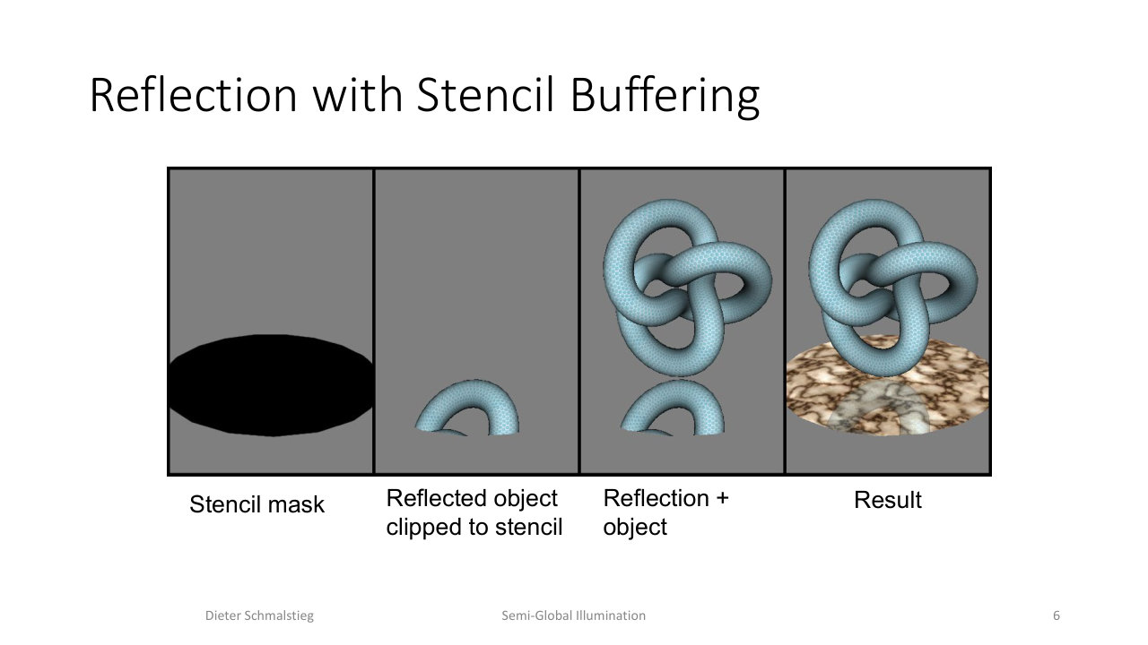
L09_Pg-006: Stencil-based reflection in four steps - write the mirror shape into the stencil, draw the mirrored object clipped to the stencil, then the normal object and the mirror surface on top.

Algorithm:

1. Clear the stencil buffer to zero.
2. Render the mirror surface, writing 1 into the stencil (stencil test off, stencil write always).
3. Render the mirrored geometry (scaled by $(1,1,-1)$) with stencil test enabled, only writing where stencil is 1.
4. Render the mirror surface again, this time as a semi-transparent surface (e.g. 50% blend).
5. Render the unmirrored scene normally.

The stencil test happens after the fragment shader and before depth blending in the fixed-function raster pipeline, so it cheaply masks pixels without doing extra shader work.

Caveats

• Handedness flips under the mirror transform; you must flip the winding order of front faces when rendering the reflected geometry.
• Intersection with the mirror plane requires clipping; otherwise geometry that pokes through the mirror creates artifacts.
• More advanced shader-based reflections can fade reflected color with distance from the reflector, apply distorted texture coordinates for fuzzy reflections, and add refraction by rendering the part of the scene below the mirror plane into a separate texture and sampling it with refracted coordinates (Valve’s water in Half-Life 2 is the canonical example).

---

3. Screen-Space Reflections

Even with RTX hardware, fully ray-traced reflections are expensive. Screen-space reflections (SSR) cheat: they reuse the deferred renderer’s color and depth buffers to approximate reflections by ray-marching in screen space.

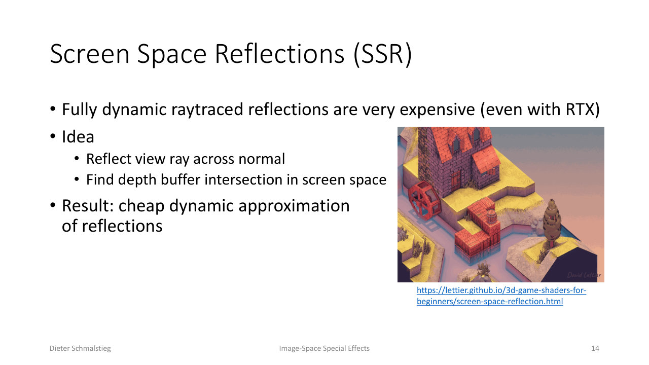
L09_Pg-014: SSR reflects the view ray across the surface normal and finds where that reflection ray intersects the depth buffer - a cheap dynamic reflection.

The algorithm per pixel:

1. Read the reflection map - a per-pixel scalar (precomputed from material roughness) that decides how much SSR to apply. Zero pixels skip SSR entirely.
2. Reflect the view ray across the surface normal at this pixel, giving a reflection direction in view space.
3. Project that reflection direction into screen space.
4. Ray-march along that screen-space direction, checking each step against the depth buffer.
5. If the ray’s depth crosses the depth buffer, the intersection point is the reflection sample - read its color from the color buffer.

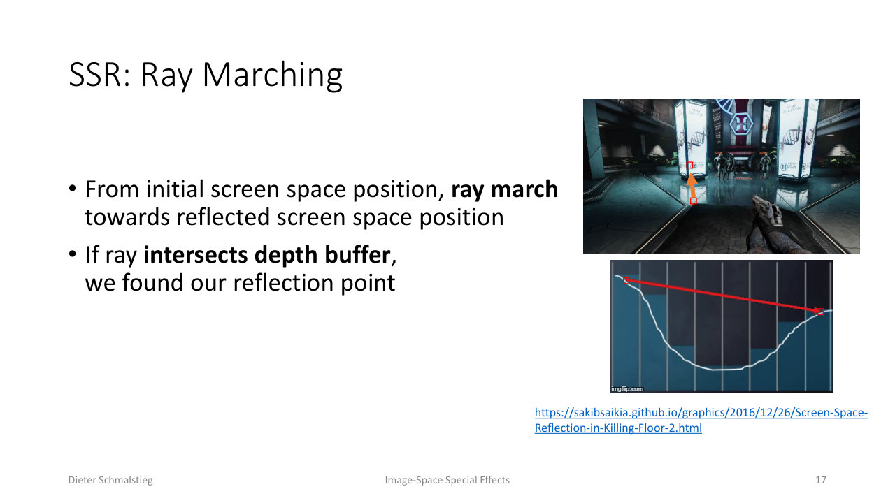
L09_Pg-017: From the initial screen position, march along the reflected screen-space direction until the ray's depth exceeds the depth buffer at that pixel.

To pin down a precise intersection, a fixed step size is followed by a binary search between the last-outside and first-inside samples, giving sub-step accuracy without many extra texture taps.

SSR Limitations

SSR’s screen-space nature creates fundamental failure modes:

• Viewer-facing reflections disappear because the reflected geometry is behind the camera and no longer in the buffer.
• Reflections outside the viewport disappear for the same reason.
• Back faces cannot be reflected because the G-Buffer stores only the nearest visible front face.
• Depth complexity: thin or layered geometry behind the visible front face cannot be reflected, since only the front-most depth is recorded.
• Flickering, holes, and temporal artifacts appear as the camera moves and reflected pixels enter or leave the screen.

Production engines mitigate these by blending SSR with cubemaps or baked reflections in unreliable regions, applying TAA-style temporal filtering to smooth flickering, blurring rough-material reflections, and capping the ray’s world-space length to prevent far-away noise.

---

4. Transparency: Order Matters

Alpha blending is order-dependent. The over operator $C_{out}={\alpha }_s{C}_s+(1-{\alpha }_s)C_d$ only gives the right answer if surfaces are blended back to front.

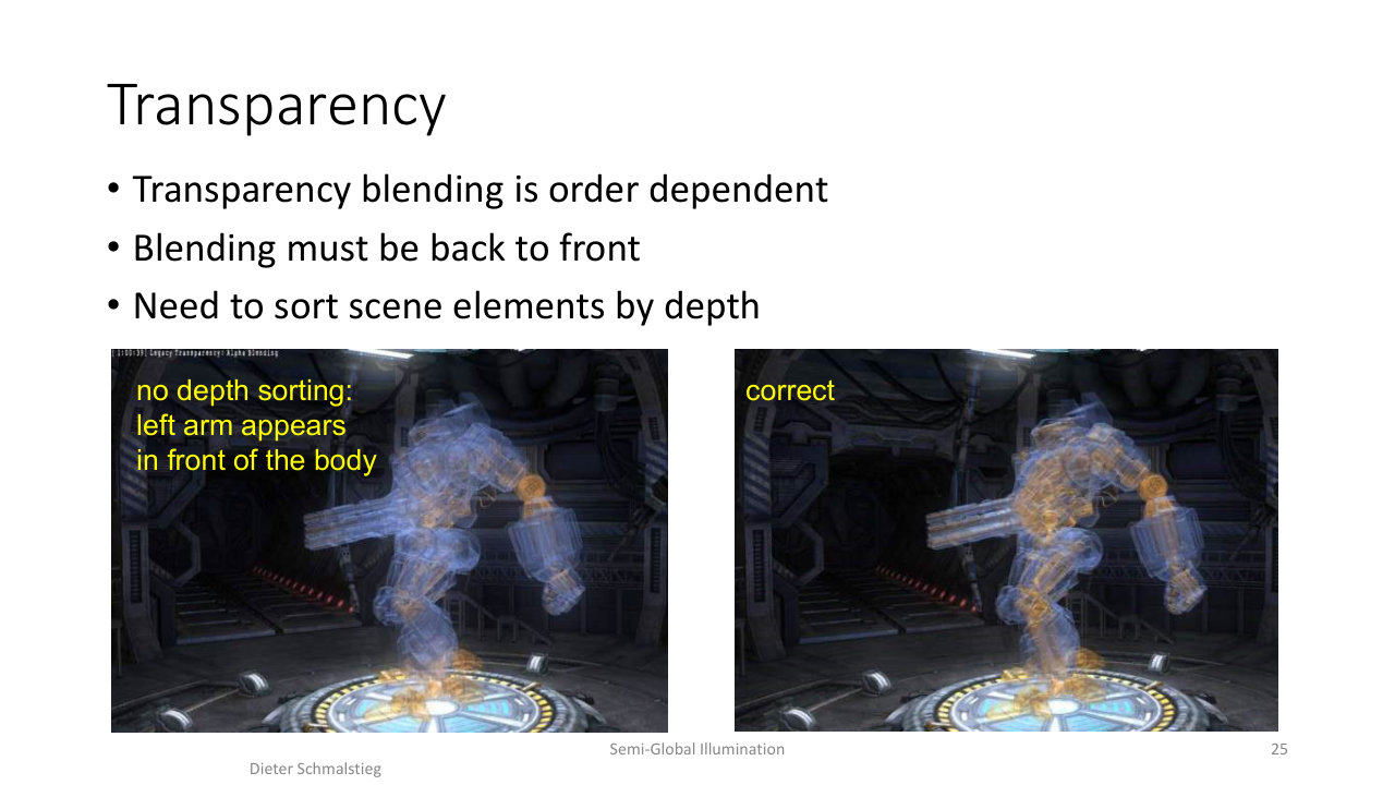
L09_Pg-025: Without depth sorting, the left arm appears in front of the body because its triangles happened to be drawn after the body; with sorting, the layering is correct.

There are three standard approaches to producing the right order.

Explicit Depth Sorting

Sort triangles by depth on the CPU (or with a compute pass) before submitting them. Pros: standard primitive order, no shader changes. Cons: writing the sorted order to memory is expensive, and per-triangle sorting fails for cyclic overlap and intersecting triangles. You can split intersecting triangles (ugly, brittle) or sort per fragment instead.

Depth Peeling

[Everitt 2001] is the canonical interactive order-independent transparency (OIT) algorithm.

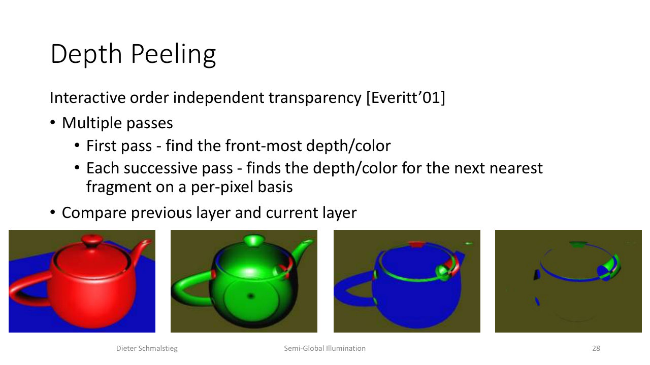
L09_Pg-028: Depth peeling renders the scene n times, each pass extracting the next-nearest fragment by comparing depth to the previous layer.

Each pass renders the scene and keeps the nearest fragment whose depth is greater than the previous layer’s depth. After $n$ passes you have $n$ ordered depth layers per pixel, ready to blend back to front. Dual depth peeling peels one layer from the front and one from the back simultaneously per pass, halving the number of passes to $n/2+1$.

The cost: each peel re-renders the whole scene, giving $O(\text{triangles}\times \text{overdraw})$ geometry overhead.

Deep Framebuffer (Per-Pixel Linked Lists)

The modern OIT approach: write every fragment produced during rasterization into a global list, then sort and blend later. Historically called the A-buffer (accumulation buffer).

Two auxiliary buffers are needed:

• Fragment and link buffer: a large flat buffer storing fragment data (color, depth, next-pointer) for every fragment, with an atomic counter for next-index allocation.
• Start offset buffer: screen-sized texture holding the index of the most recently written fragment for each pixel, initialized to -1 (end-of-list sentinel).

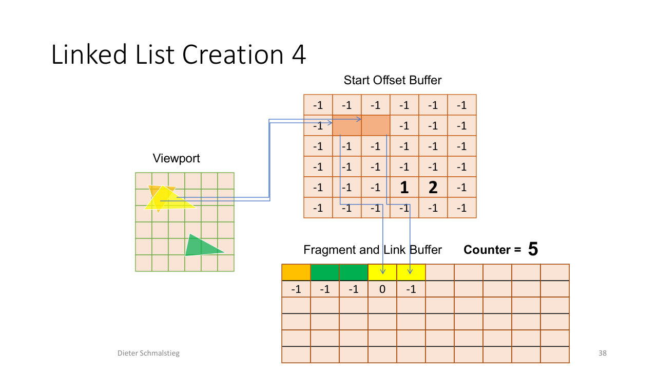
L09_Pg-038: Linked-list creation in progress - each new fragment is appended to the head of its pixel's list, with the old head index recorded as the next pointer.

The fragment shader appends each fragment with an atomic operation, pushes the new entry onto the head of the per-pixel list, and stores the previous head index as its next pointer. Traversal is a fullscreen quad (or compute shader) that, for each pixel, walks the linked list, sorts the fragments into a small temp array by depth, and blends them back to front.

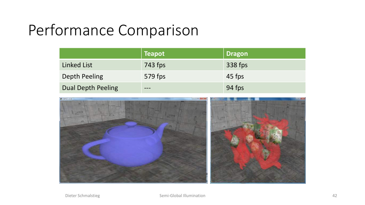
L09_Pg-042: For a heavily transparent dragon scene, linked-list OIT runs ~3.5x faster than depth peeling because it amortizes the geometry pass.

Linked lists win when overdraw is high because the scene is rasterized only once, regardless of how many transparent fragments end up at a pixel.

---

5. Shadows as a Global Effect

Shadows are an important visual cue: they tell us the relative position of objects and the position of the light, and without them objects look like they are floating.

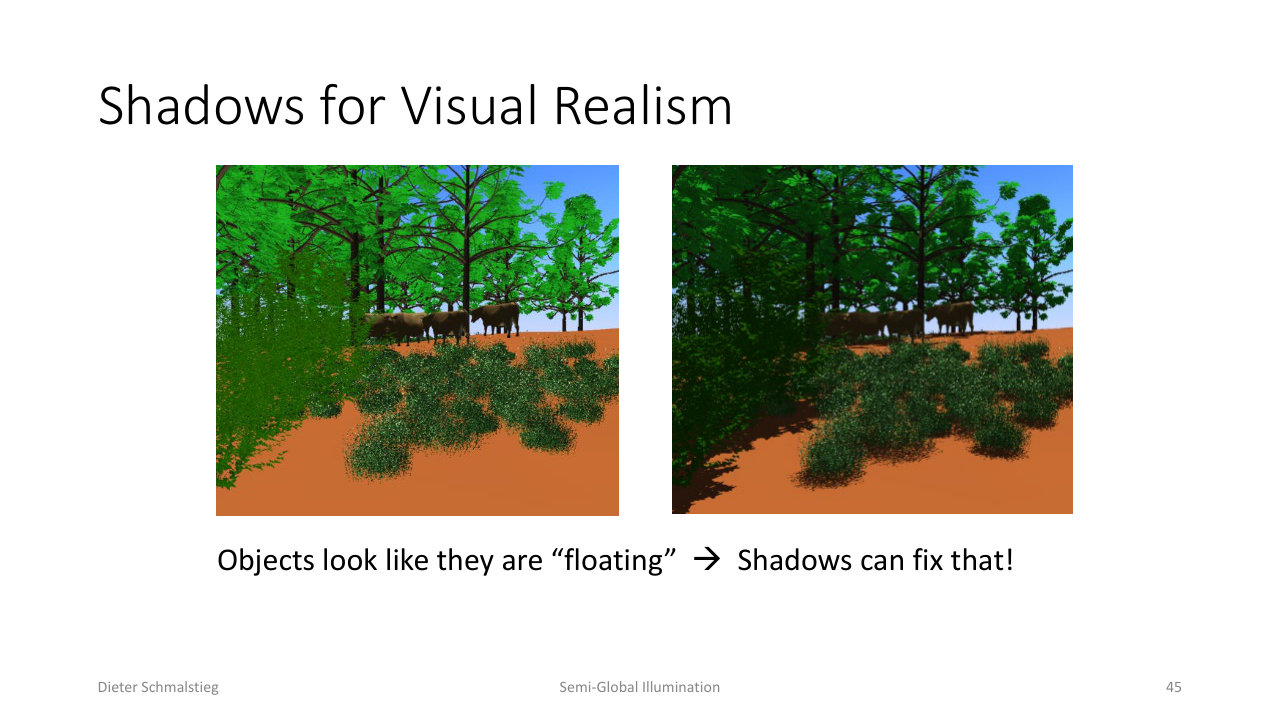
L09_Pg-045: Without shadows, characters and bushes float over the ground; with shadows, they sit on the surface.

A shadow is a non-local interaction between a light source, the receiver (the surface being shaded), and an occluder (the object blocking light from reaching the receiver). Even regular shading can be thought of as a kind of pseudo self-shadowing - the $\max (\mathbf{N}\cdot \mathbf{L},0)$ Lambert factor is just “fully occluded when the surface faces away from the light.”

Shadow Geometry

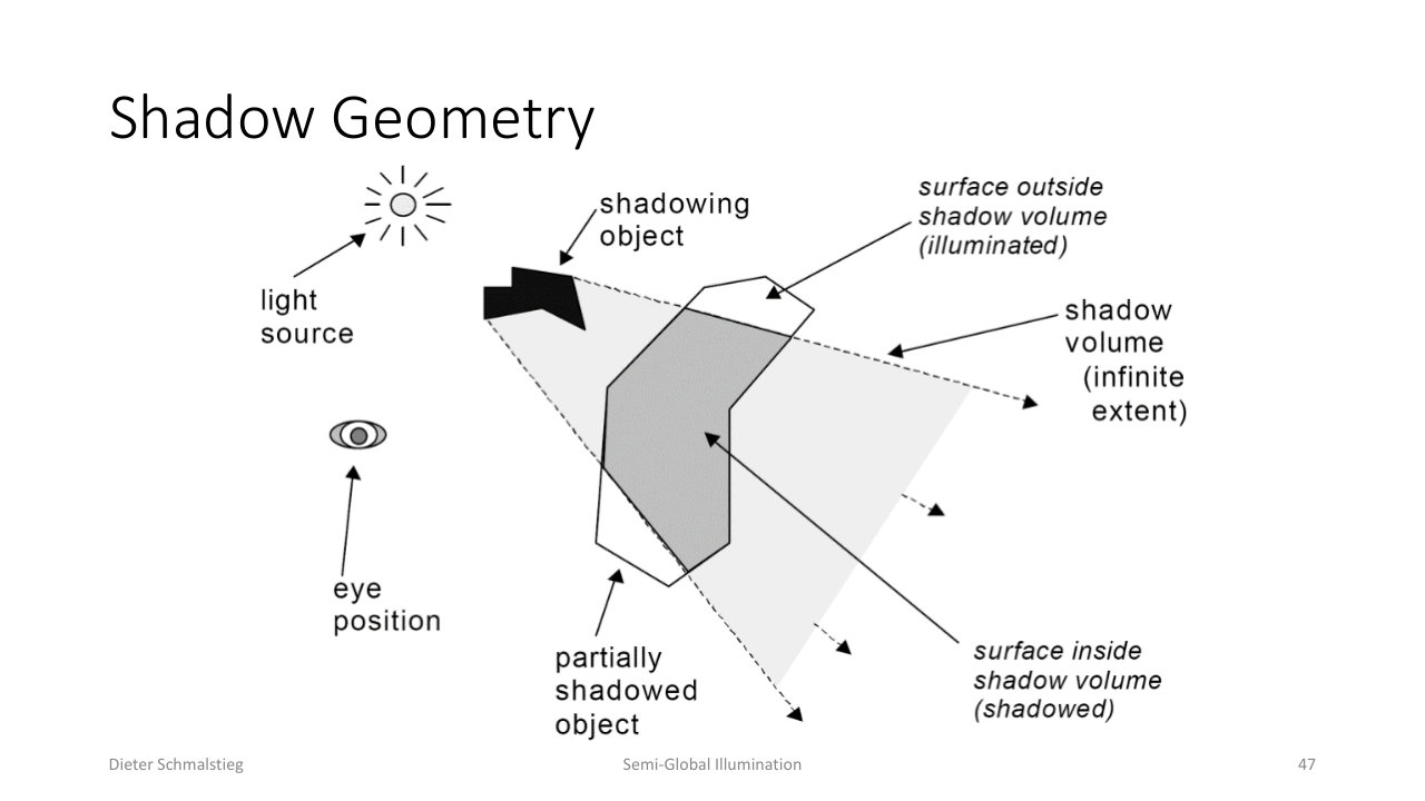
L09_Pg-047: A shadowing object carves a shadow volume - surfaces inside are shadowed, surfaces outside are illuminated, surfaces partially inside are partially shadowed.

The geometric structure is a shadow volume: the region of space behind the occluder, relative to the light, that the light cannot reach.

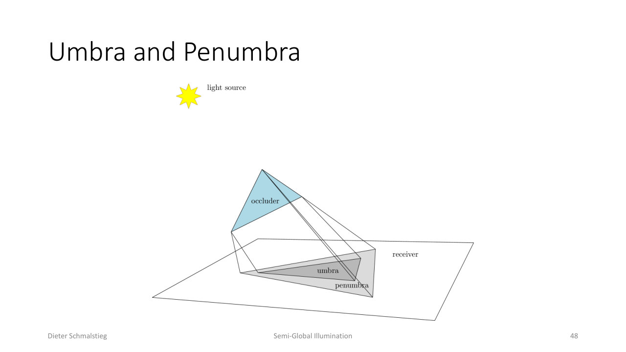
L09_Pg-048: An area light produces an inner umbra (fully occluded) surrounded by a penumbra (partially occluded).

For an area light, the shadow has structure: the umbra is fully occluded (no part of the light reaches it), the penumbra is partially occluded (some part of the light is blocked). Point lights produce only umbra; their shadows are hard-edged. Most real-time techniques approximate area-light shadows by softening point-light shadow maps with filtering.

Why Shadows Are Hard

Shadows are a global illumination problem because deciding whether a point is in shadow requires knowing about geometry elsewhere (the occluder). In an online rendering pipeline that processes one triangle at a time, the global information is not available.

The two-pass workaround is universal: in pass 1, compute and store global shadow information into a buffer (a depth map, a stencil mask, or precomputed light data); in pass 2, render the scene using that buffer to look up shadowing per pixel.

---

6. Approximate Shadows

For very cheap “good-enough” shadows, two tricks predate proper shadow algorithms.

Hand-drawn approximate geometry: a few low-poly meshes (a flat disc under a car, a polygonal blob under Lara Croft) suggest contact. Perceptual studies show shape is not very important to the cue; presence is.

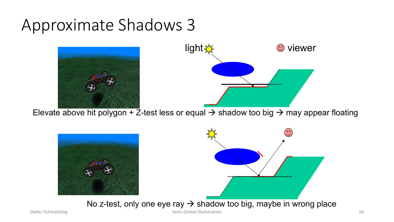
L09_Pg-056: Naive blob shadows either z-fight with the ground (blend at hit polygon), float above it (elevate + z-test less-or-equal), or sit in the wrong place (no z-test).

Projected dark polygon: cast a ray from the light through the object centre, hit the ground, and blend a dark texture there. The hard part is z-fighting: blending at exactly the hit depth produces quantization artifacts, elevating above the ground makes the shadow appear to float, and skipping z-test entirely puts the shadow wherever the projection lands regardless of geometry.

---

7. Planar Projected Shadows

The first principled method, due to Blinn 1988: project the shadow caster onto a plane using a projective matrix derived from the light position, then draw the projected geometry darkly.

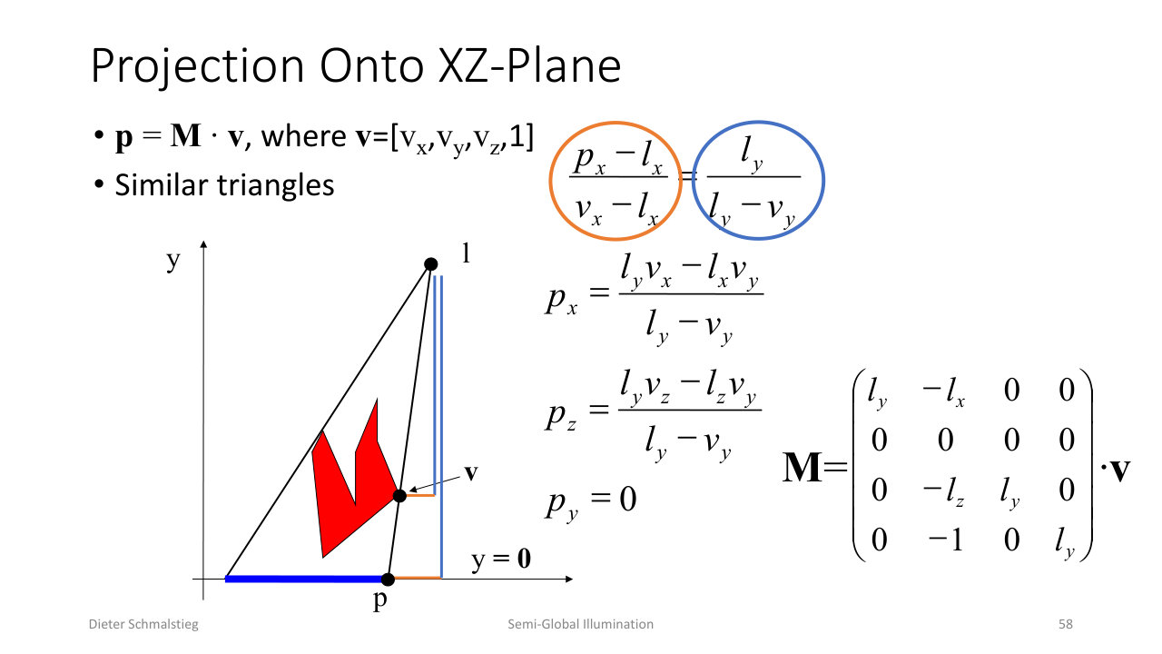
L09_Pg-058: Projection onto the XZ-plane from a light $\mathbf{l}$ comes out of similar triangles, giving $p_x = (l_y v_x - l_x v_y)/(l_y - v_y)$, $p_y = 0$, and an analogous expression for $p_z$.

For a light at $\mathbf{l}$ and a vertex at $\mathbf{v}$, the projection onto a general plane $\mathbf{n}\cdot \mathbf{p}+d=0$ is

$\mathbf{p}=\mathbf{l}-\frac{d+\mathbf{n}\cdot \mathbf{l}}{\mathbf{n}\cdot (\mathbf{v}-\mathbf{l})}(\mathbf{v}-\mathbf{l})$

which can be written as a $4\times 4$ matrix applied to the vertex.

Pros: arbitrary shadow casters, very cheap. Cons: only planar shadow receivers (one plane at a time), no self-shadowing, and several common artifacts.

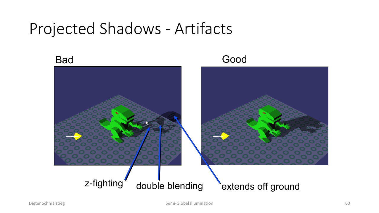
L09_Pg-060: Projected shadow artifacts - z-fighting with the receiver, double blending where projected triangles overlap, and shadow extending off the ground plane.

The classic artifacts:

• Z-fighting between the projected shadow and the receiver plane.
• Double blending where the projected silhouette folds onto itself, darkening the overlap.
• Shadow extending off the receiver when the projected geometry continues past the plane’s edge.

The standard fix uses a stencil buffer: draw the receiver plane writing 1 into stencil, draw the projected shadow only where stencil is 1 (which also writes 0 back), so each shadow pixel is blended exactly once and no shadow extends off the plane. GLQuake (1997) was the first game to ship this technique.

---

8. Shadow Mapping

Shadow mapping is the modern dominant shadow technique. The idea:

1. Pass 1: render the scene from the light’s point of view, storing only the depth buffer. This is the shadow map - the depth of whatever the light “sees” first in each direction.
2. Pass 2: render the scene normally from the camera. For each pixel, transform its position into the light’s coordinate frame, look up the shadow map at that position, and compare depths.

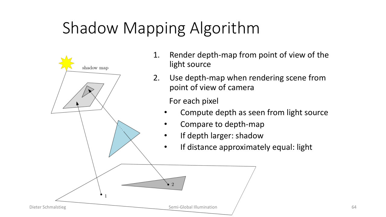
L09_Pg-064: For each camera pixel, compute its depth as seen from the light, compare to the shadow map; if the camera-pixel depth is greater, the pixel is in shadow.

If the camera-pixel’s light-space depth is greater than the shadow map’s value, something else was nearer the light at that ray - the pixel is in shadow. If the depths are approximately equal, the pixel itself was visible to the light - it is lit.

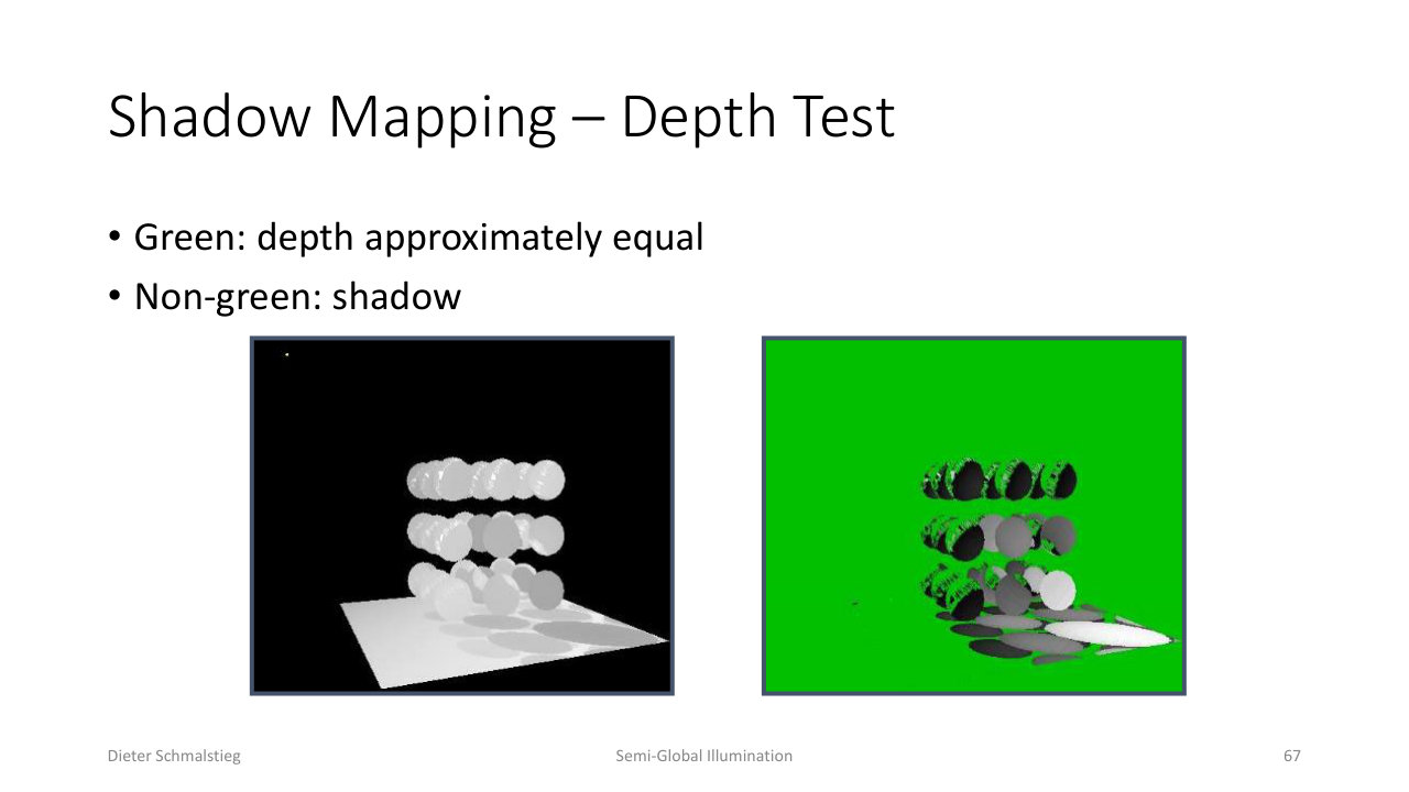
L09_Pg-067: Pixels whose camera-light depth matches the shadow map are coloured green (lit); the rest are darker (shadowed).

Shadow mapping inherits the strengths and weaknesses of any sampled-buffer technique: it is fast (one extra render pass) and independent of scene complexity, supports self-shadowing, and works for anything that can be rendered. But it has serious aliasing problems and needs careful bias tuning.

Aliasing

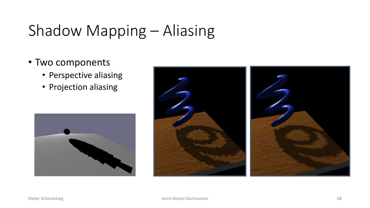
L09_Pg-068: Shadow-map aliasing has two components - perspective aliasing (camera-space texel resolution) and projection aliasing (shadow-map texel resolution under glancing angles).

Two distinct aliasing problems coexist:

• Perspective aliasing: when the camera is close to a shadowed surface, each shadow-map texel covers many pixels in image space. The shadow becomes blocky.
• Projection aliasing: when the light hits the surface at a steep glancing angle, each shadow-map texel covers a long stretch of surface. Shadow texels appear stretched.

Percentage Closer Filtering

Naive bilinear filtering of the shadow map gives wrong answers, because averaging depth values produces a meaningless interpolated depth that may not match anything in the scene. The right approach is percentage closer filtering (PCF): for each shadow-map sample in the kernel, compare to the surface depth first, then filter the binary lit/shadow result.

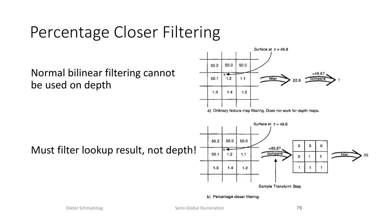
L09_Pg-076: PCF filters the boolean lit/shadow result of per-texel comparison, not the depth values themselves; the example averages 5 of 9 lit samples to give 0.55 visibility.

PCF gives smoother shadow edges in a single pass - much cheaper than a separate screen-space blur - and is supported as a hardware sampler in modern APIs.

Depth Precision and Bias

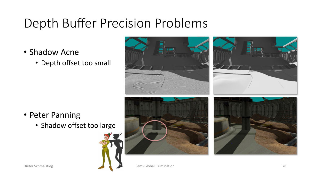
L09_Pg-078: Too small a depth offset gives shadow acne (every lit surface flickers in self-shadow); too large gives Peter Panning (shadow detaches from the object).

Comparing depth values exactly is impossible because of quantization. Two failure modes:

• Shadow acne (depth offset too small): self-shadow patterns appear on lit surfaces, because each surface point’s stored depth is slightly different from its computed depth.
• Peter Panning (depth offset too large): the shadow detaches from its caster, making the object look like it floats.

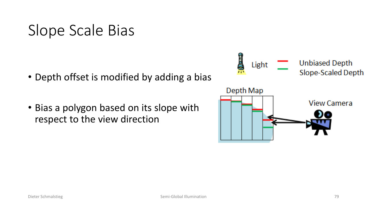
L09_Pg-079: Slope-scale bias adjusts the depth offset per polygon based on its slope relative to the light, applying a larger offset for steep angles where quantization is worse.

Slope-scale bias adapts the offset per polygon based on its slope to the light direction. Steep polygons need more bias; nearly head-on polygons need almost none. Combined with PCF this is enough for most scenes.

Other practical optimizations:

• Optimize the shadow frustum by fitting near and far planes to the intersection of the light frustum with the scene bounding box, minimizing wasted depth range.
• Cascaded shadow maps (CSM) for large outdoor scenes.

Cascaded Shadow Maps

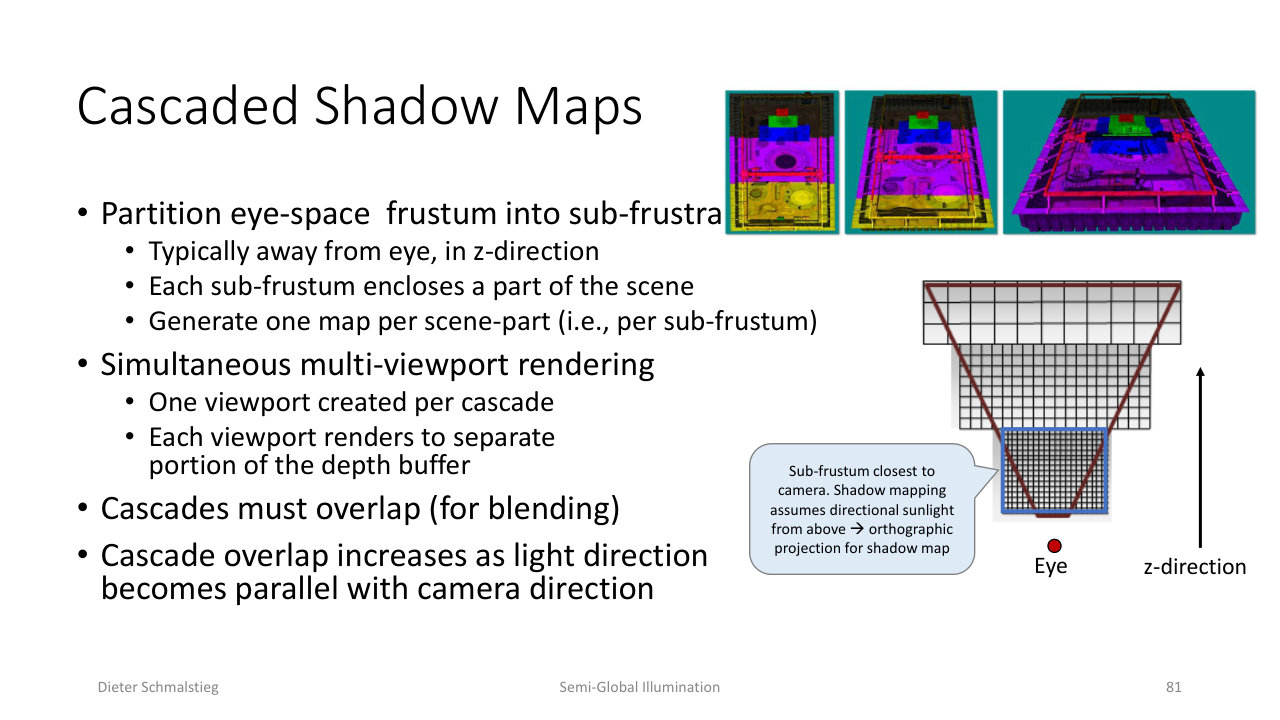
L09_Pg-081: CSM partitions the eye-space frustum into cascading sub-frusta along z, with a separate shadow map per cascade - nearby cascades cover little area at high resolution, far cascades cover more at lower resolution.

For a directional light (sun), one shadow map covering the whole view is necessarily low-resolution at close range, where blocky shadows are most visible. CSM splits the eye-space view frustum into $N$ depth slices, generates one shadow map per slice in light space, and uses the appropriate cascade per pixel.

The cascade split distances are typically a blend of logarithmic and linear partitions:

$z_i=\lambda n{\left(\frac{f}{n}\right)}^{i/N}+(1-\lambda )\left(n+\frac{i}{N}(f-n)\right)$

with $\lambda \approx 0.9$ giving mostly logarithmic spacing for natural perceptual distribution, plus a small linear term so transitions are not too abrupt. Multi-viewport rendering generates all $N$ cascades in one pass into different regions of a single depth attachment.

Omni-Directional Shadow Maps

Standard shadow mapping handles spot and directional lights, which have a single forward direction. For omni-directional point lights you need to cover the full $4\pi$ steradian sphere of directions.

The cube-map approach uses six shadow maps, one per cube face - accurate but expensive (six extra render passes).

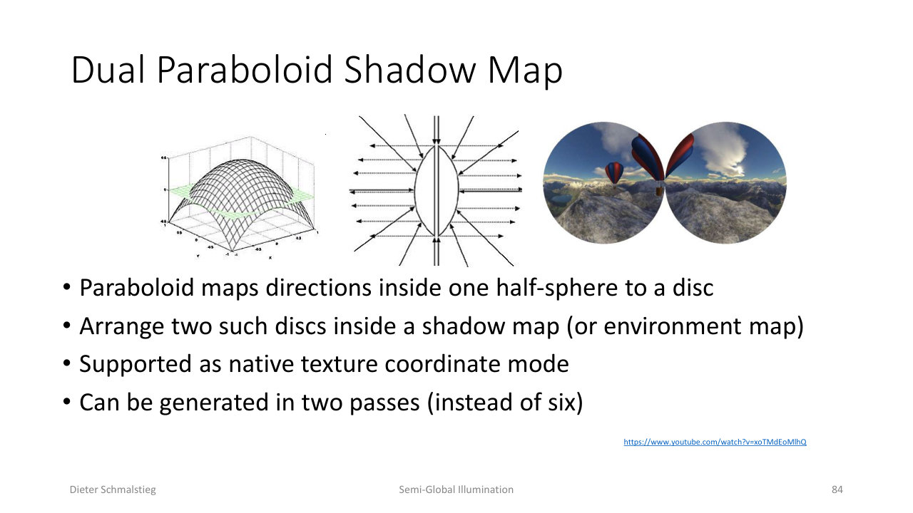
L09_Pg-084: A dual paraboloid shadow map projects each hemisphere onto a disc - two passes instead of six, supported by native texture-coordinate hardware.

The dual paraboloid shadow map is the cheaper alternative: a paraboloid surface maps every direction inside a hemisphere onto a disc. Two such discs, one for each hemisphere, fit inside a single texture. Generation needs only two passes (one per hemisphere) instead of six.

Shadow Mapping Summary

• Fast - one extra rendering pass.
• Independent of scene complexity, no extra shadow geometry.
• Supports self-shadowing (with proper bias).
• Sometimes can reuse depth from other passes.
• Problematic for omnidirectional lights (cubemap or paraboloid needed).
• Biasing tuning needed to balance light leaks and shadow acne.
• Jagged edges from aliasing, mitigated by PCF and CSM.

---

9. Shadow Volumes

The alternative shadow technique, due to Crow 1977 and made famous by Doom 3, is to compute shadow boundaries geometrically instead of sampling them.

For each shadow caster and light, build the shadow volume: extrude the caster’s silhouette edges away from the light, capping the volume with the light-facing polygons (light cap) and the away-facing polygons projected to infinity (dark cap).

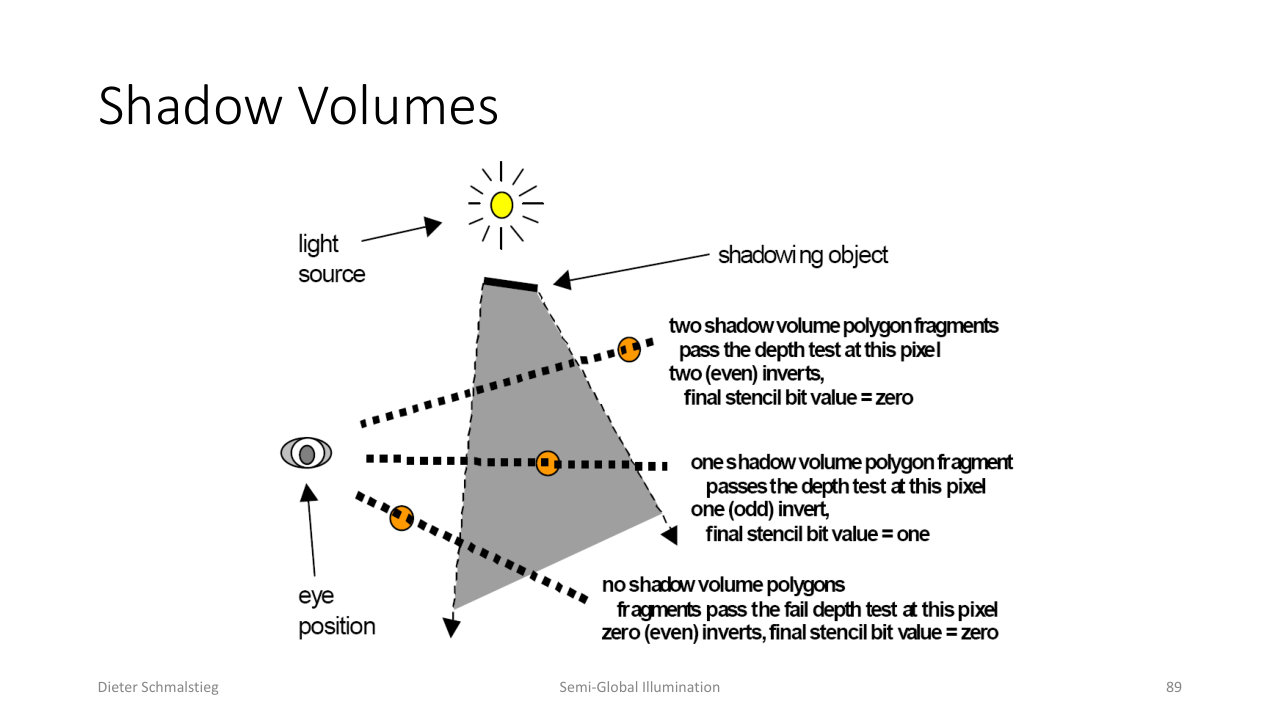
L09_Pg-087: For each pixel, count how many shadow-volume polygon fragments pass the depth test along the view ray. An odd count means the pixel is inside the volume (shadowed), even means outside (lit).

The shadowing test for each pixel:

1. Fill the depth buffer with the lit scene.
2. Disable depth writes.
3. Render the front faces of the shadow volume, incrementing the stencil where the depth test passes.
4. Render the back faces of the shadow volume, decrementing the stencil where the depth test passes.
5. Pixels with stencil $=0$ at the end are lit; non-zero are in shadow.

The logic, geometrically: each entry into the shadow volume between the camera and the rendered pixel adds $+1$ (front face passes depth test); each exit subtracts $-1$ (back face passes depth test). Inside the volume the sum is positive; outside it cancels back to zero.

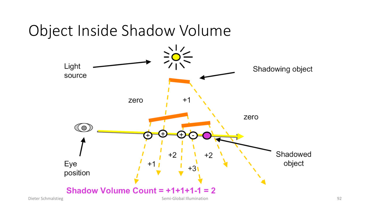
L09_Pg-090: For an object inside the shadow volume, the front-face increment outnumbers the back-face decrement by 1 - the stencil value is non-zero, so the pixel is shadowed.

Depth-Pass vs Depth-Fail

The default scheme (depth-pass, or “Carmack’s z-pass”) fails when the camera is inside the shadow volume - front faces that would normally increment the stencil are clipped by the near plane, throwing off the count.

The fix (depth-fail, or “Carmack’s reverse”): increment the stencil on back faces that fail the depth test, decrement on front faces that fail. This counts shadow-volume crossings behind the pixel rather than in front, which is robust even when the camera is inside the volume. It costs extra geometry (you need a closed dark cap at infinity using projective vertices with $w=0$) but is the safe choice.

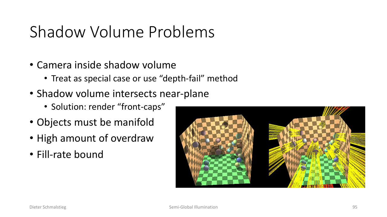
L09_Pg-093: Shadow volumes need closed-manifold meshes, can produce extreme overdraw, and are fill-rate bound - the right image visualizes the wireframe of just the shadow volume polygons.

Shadow Volume Problems

• Closed-manifold geometry required (otherwise silhouette extraction breaks).
• Cost hard to predict: shadow-volume geometry grows with caster silhouette length.
• Bandwidth heavy: every shadow volume face has to be rasterized into the stencil buffer.
• Extreme overdraw: shadow-volume polygons often cover large screen areas; fill rate dominates.

Comparison: Volumes vs Mapping

Aspect	Shadow Volumes	Shadow Mapping
Geometry requirement	Closed manifolds only	Anything renderable
Cost predictability	Hard (depends on silhouette)	Predictable (one extra pass)
Memory/bandwidth	High (stencil-heavy)	Moderate (one depth texture)
Sampling artifacts	None	Yes (aliasing, bias tuning)
Hardware support	Stencil ops	PCF samplers built in

Shadow mapping dominates modern engines because the artifacts are well-understood and the cost is bounded, while shadow volumes remain a textbook example of an exact geometric approach.

---

10. Environmental Lighting and Ambient Occlusion

Everything above assumes a known directed light. The other half of the picture is environmental lighting: indirect light bouncing in from all directions of the surrounding environment.

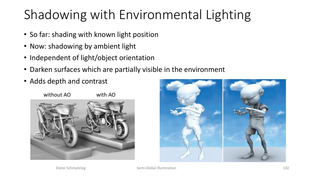
L09_Pg-099: Ambient occlusion darkens surfaces partially blocked from environmental light - independent of light direction, it adds depth and contrast in corners, crevices, and contact areas.

Ambient occlusion (AO) is the cheap approximation: instead of computing every bounce, darken surfaces in proportion to how much of the surrounding hemisphere is blocked. AO depends only on geometry, not on light direction, and dramatically improves the perceived depth and grounding of objects.

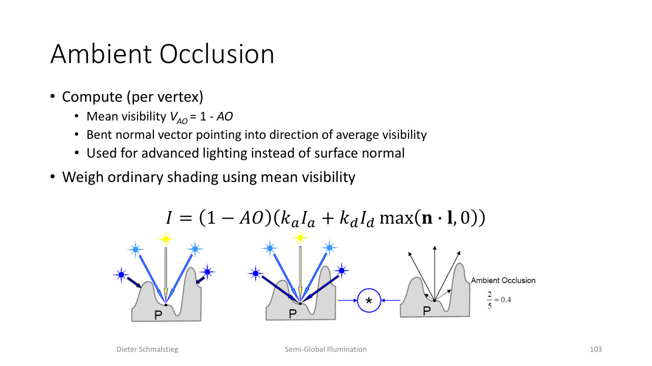
L09_Pg-100: AO weighs the standard shading by $(1 - AO)$ - a fully unoccluded surface uses normal lighting; a deep crevice with $AO \to 1$ goes dark.

The basic AO equation modifies regular shading by a visibility scalar:

$I=(1-AO)(k_a{I}_a+k_d{I}_d\max (\mathbf{N}\cdot \mathbf{L},0))$

Per vertex, precompute the mean visibility $V_{AO}=1-AO$ by casting $n$ rays into the upper hemisphere and counting blocked rays $m$, then $V_{AO}=1-m/n$. A cosine-weighted distribution accounts for Lambert’s law. A bent normal pointing toward average visibility can be stored as well, and used in place of the geometric normal for ambient lighting calculations.

The catch: ray-casting from every vertex of every static asset is expensive. For dynamic geometry it is infeasible offline.

Screen-Space Ambient Occlusion

The screen-space approximation observes that the depth buffer is already a low-fidelity approximation of the scene’s surroundings.

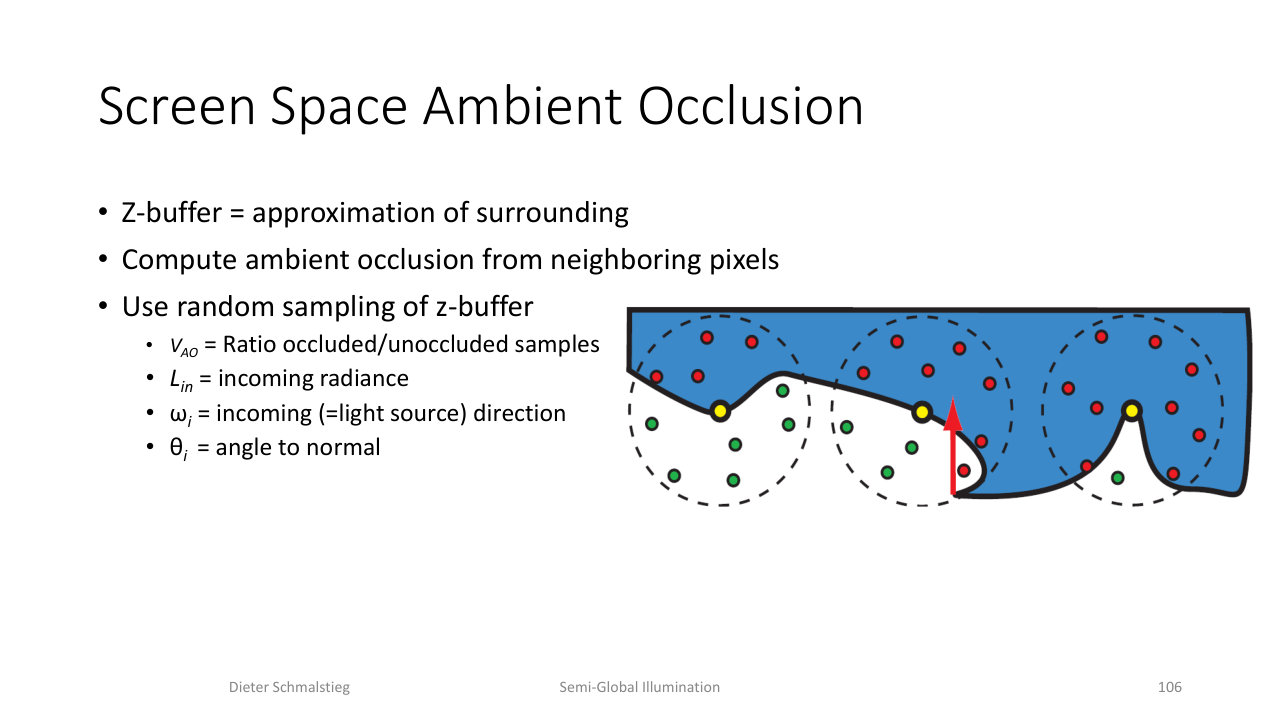
L09_Pg-103: SSAO samples the depth buffer in a hemisphere around each pixel and counts samples whose depth lies "inside" the surface as occluded.

For each pixel:

• Generate a random set of sample positions in a hemisphere around the pixel, oriented by the surface normal.
• For each sample, project to screen space and look up the depth buffer.
• If the sample’s depth is “behind” the depth buffer (inside the scene), it counts as occluded.
• The fraction of occluded samples becomes the per-pixel AO.

SSAO is a postprocess: cost depends on screen resolution and sample count, not scene polygon count. It runs entirely on the G-Buffer, fits inside the deferred-shading pipeline, and is dynamic (animated objects automatically contribute).

Screen-Space Directional Occlusion and a First Bounce

SSAO uses scalar occlusion only - it darkens equally regardless of where the surrounding geometry is. Screen-space directional occlusion (SSDO) considers direction: a sample is treated as an occluder of incoming light from a specific direction, so light coming from unblocked directions still hits the surface.

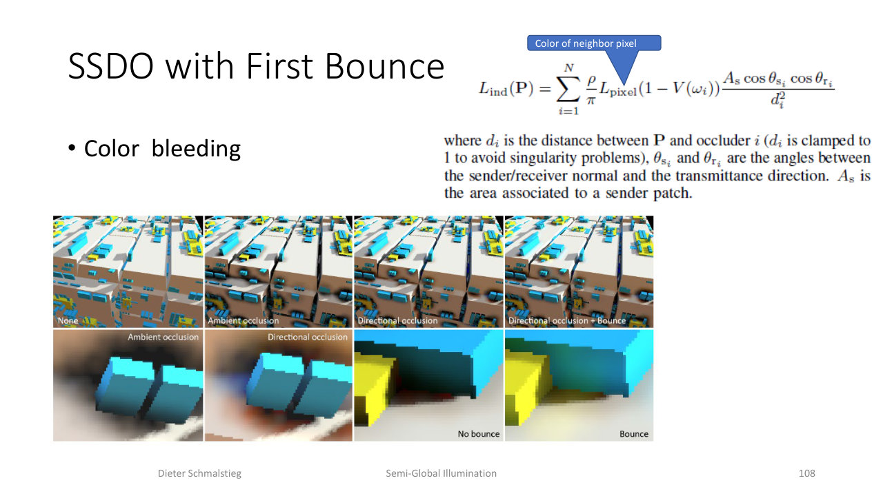
L09_Pg-105: SSDO with first bounce takes the color of each occluder pixel as a small radiating patch, giving cheap color bleeding (red wall casting red onto nearby spheres).

The further extension: each detected occluder is treated as a small Lambertian patch radiating the color already in the color buffer at that pixel. The bounced contribution at receiver $\mathbf{P}$ becomes

$L\ast \text{ind}(\mathbf{P})=\sum \ast {i=1}^N\frac{\rho }{\pi }L\ast \text{pixel}(1-V({\omega }_i))\frac{A_s\cos \theta \ast s\ast i\cos \theta \ast r_i}{d_i^2}$

where $A_s$ is the sender patch area and $d_i$ is the sender-receiver distance (clamped to 1 to avoid singularities). The result is cheap color bleeding - red walls tint nearby spheres red, green floors give a green wash to objects sitting on them - at the cost of one extra sampling pass per pixel.

In Crysis this is used to give dynamic objects (which receive but do not contribute to GI) plausible bounce light from static walls and terrain that do contribute. When the light direction changes, the dominant bounce shifts naturally.

---

Applied Exam Focus

• Semi-global recipe: local shading everywhere, global effects (reflection, transparency, shadows, AO) computed selectively in a two-pass technique that writes an auxiliary buffer then reads it during shading.
• Stencil-based planar reflection: render mirror into stencil = 1, render mirrored geometry clipped to stencil 1, render mirror semi-transparent, render unmirrored scene. Adjust front-face winding because reflection flips handedness; clip against the mirror plane.
• Screen-Space Reflections: reflect view ray across surface normal, ray-march the depth buffer in screen space, binary-search the intersection. Cheap but fails for back faces, off-screen geometry, viewer-facing surfaces, and gives flickering at depth complexity boundaries.
• Transparency is order-dependent (back-to-front blending). Three approaches: explicit sort, depth peeling ($n$ render passes, one per layer; dual variant halves to $n/2+1$), per-pixel linked lists (every fragment appended via atomic counter, traversal sorts then blends).
• Shadow math: a shadow is a global interaction between light, occluder (blocker), and receiver. Area lights give umbra + penumbra; point lights give only umbra.
• Planar projected shadows: project the caster onto a plane through a 4x4 projection matrix; combine with a stencil mask to avoid double blending and z-fighting. Only one planar receiver per shadow; no self-shadowing.
• Shadow mapping: pass 1 renders depth from the light’s view (the shadow map); pass 2 looks up per pixel and compares depths. Use slope-scale bias to balance shadow acne vs Peter Panning; use PCF to filter the comparison result, not the depth values.
• Cascaded shadow maps: partition the camera frustum into depth slices, generate one shadow map per slice in light space, blend across cascade boundaries; split distances are a $\lambda$-blend of logarithmic and linear ($\lambda \approx 0.9$).
• Omnidirectional shadows: cube-map (six passes, accurate) or dual paraboloid (two passes, native texture-coord mode).
• Shadow volumes: extrude silhouette edges away from the light; count front-face increments and back-face decrements in the stencil along each view ray. Depth-pass scheme is cheap but fails inside the volume; depth-fail (Carmack’s reverse) increments back-faces that fail the depth test, robust everywhere but needs closed front/back caps at infinity.
• Ambient Occlusion: precomputed mean visibility per vertex via raycasting into the upper hemisphere, applied as $(1-AO)$ multiplier on shading. SSAO does the same in screen space using the depth buffer as a proxy for geometry.
• SSDO: directional version of SSAO that considers which incoming directions are blocked; the bounce extension uses the color of each occluder pixel as a small radiating patch, giving cheap color bleeding.

Self-Check

1. Why does stencil-based planar reflection require adjusting the winding order of front faces when rendering the mirrored geometry?

Answer

Scaling geometry by $(1,1,-1)$ across the mirror plane flips handedness, which reverses the winding order of every triangle. Without compensating, every triangle that used to face the camera now faces away and gets culled by the standard back-face culling rule. Flipping the winding order (or equivalently inverting the cull-face state) restores correct visibility.

2. What information does a screen-space reflection actually trace, and what failure modes follow from that?

Answer

SSR reflects the per-pixel view ray across the surface normal and ray-marches the result against the depth buffer until it finds an intersection with whatever the scene rendered into the color buffer. Because it only knows what is on screen, it cannot reflect surfaces that are off-screen, behind the camera, hidden behind the front-most depth (back faces, layered geometry), or anything outside the viewport. The result is missing or flickering reflections at silhouettes and depth boundaries.

3. Compare depth peeling and per-pixel linked lists as solutions to order-independent transparency.

Answer

Depth peeling re-renders the entire scene once per transparency layer, each pass extracting the next-nearest fragment by comparing depths to the previous layer’s output. Per-pixel linked lists rasterize the scene once and append every fragment that lands on each pixel into a global linked list with an atomic counter; a separate traversal pass sorts and blends each list. Depth peeling pays $O(\text{triangles}\times \text{layers})$ in geometry cost; linked lists pay one geometry pass plus per-pixel sort and bandwidth for the fragment buffer, so for high overdraw scenes linked lists are much faster (the lecture cites ~3.5x on the dragon scene).

4. Why does shadow mapping need a bias, and what is “slope-scale bias”?

Answer

Shadow mapping compares two depth values that almost never match exactly due to quantization and rasterization differences between the light-view and camera-view passes. Without a bias, surfaces shadow themselves (shadow acne); too large a bias detaches shadows from their casters (Peter Panning). Slope-scale bias adds a depth offset proportional to the polygon’s slope relative to the light direction - steep polygons need a larger offset because adjacent depth samples differ more under quantization, while head-on polygons need almost none.

5. Why does PCF apply the depth comparison before filtering rather than after?

Answer

Filtering raw depth values produces a meaningless interpolated depth that does not correspond to any actual surface, so the subsequent comparison gives wrong shadow boundaries. PCF instead compares each individual shadow-map sample to the surface depth first, producing a binary lit/shadow value per sample, and then averages those binary results to get a smooth visibility fraction at the pixel. Modern GPUs implement this as a hardware sampler so a single texture instruction returns the filtered comparison result.

6. Why does the depth-pass shadow-volume scheme fail when the camera is inside a shadow volume, and how does depth-fail (Carmack’s reverse) fix it?

Answer

Depth-pass increments the stencil for front-faces of the shadow volume that pass the depth test. When the camera is inside the volume, the relevant front faces are behind the near clip plane and get clipped before they can increment the stencil, so the counting is off by one and lit pixels are wrongly marked as shadowed. Depth-fail instead increments back-faces of the shadow volume that fail the depth test (and decrements front-faces that fail), which counts shadow-volume crossings behind the rendered pixel rather than in front of it. This is robust even when the camera is inside the volume, at the cost of needing closed front and back caps (the back cap projected to infinity with $w=0$).

7. What does SSAO measure, and how does SSDO with first bounce extend it?

Answer

SSAO measures the scalar fraction of nearby samples in a hemisphere around each pixel whose depth lies “inside” the scene relative to the surface, approximating how much of the surrounding environment is geometrically blocked. The result is a per-pixel darkening factor applied to ambient lighting, independent of light direction. SSDO extends this to consider direction (which incoming directions are blocked), and the first-bounce extension treats each occluder pixel as a tiny radiating patch whose color is the color already in the color buffer at that pixel, producing cheap color bleeding from nearby colored surfaces.

---

Back: (y-08) Image-Space Special Effects | RTG Index | Next: (y-10) Real-Time Global Illumination