10_global_illumination - Real-Time Global Illumination

Back: (y-09) Semi-Global Illumination | RTG Index | Next: (y-11) GPU Raytracing

Mental Model First: Caching Light, Not Tracing It

Offline renderers solve the rendering equation; real-time renderers approximate it by caching pieces of the light transport ahead of time and looking those pieces up at frame time. The recurring shape is two passes: pass 1 builds a cache of light transport in the scene, pass 2 shades pixels using that cache.
Every method in this lecture is a choice about what to cache, where to cache it, and how stale the cache is allowed to be. Radiosity caches diffuse radiance per surface patch. Photon mapping caches photons in a kd-tree. Instant radiosity caches the second bounce as virtual point lights with shadow maps. Reflective shadow maps cache the first bounce in light-view pixels. Illumination probes cache directional radiance at a sparse grid of points in world or screen space. PRT caches per-vertex light-transport coefficients.
The fundamental tension is between scene complexity and light transport complexity. Static scene with static lights but moving camera lets you precompute everything (storage explodes for specular). Dynamic scene with dynamic lights lets nothing be precomputed (compute explodes). Real production systems sit in the middle: static lights and semi-static geometry, with screen-space tricks filling in detail.
The big modern result is Lumen-style hybrid caching. Different ranges in the scene update at different rates: ambient occlusion per pixel each frame, screen-space probes per pixel with temporal accumulation, world-space probes amortised over many frames, skylight at the lowest rate. Lighting latency is allowed to grow with distance because the eye notices distant flicker less.
Photon mapping and radiosity solve the problem correctly but slowly; VPL-based and probe-based methods sacrifice physical correctness for frame budget. Knowing which compromises each method makes is the lecture’s point.

1. Online vs. Offline Rendering

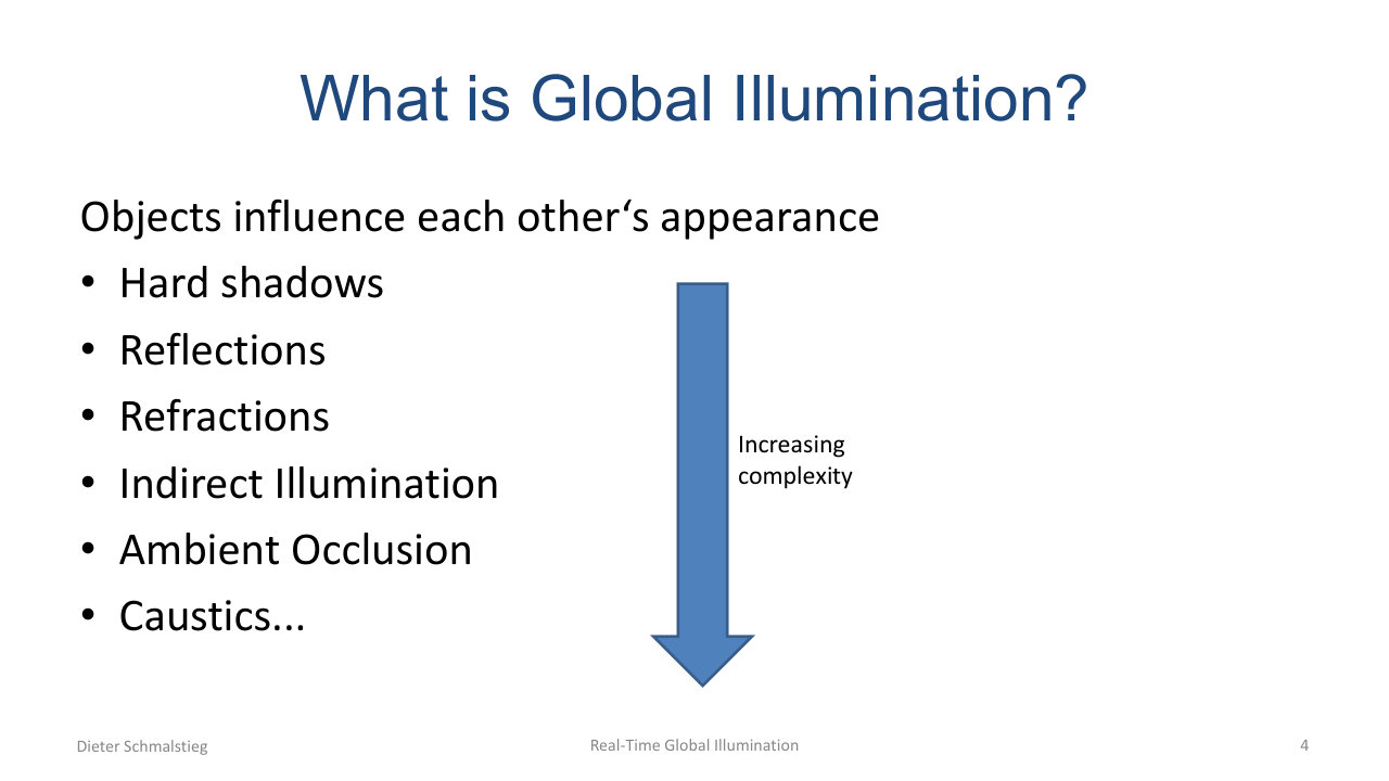
L10_Pg-04: The global effects ordered by complexity - hard shadows, reflections, refractions, indirect illumination, ambient occlusion, caustics.

In offline rendering the renderer has the whole scene in memory and is free to chase arbitrary rays around it. In online rendering the GPU streams surface fragments through a rasterisation pipeline and only sees one triangle at a time. Most of the techniques in this lecture exist because global light transport does not fit naturally into the online setting.

Global illumination means objects influence each other’s appearance. In order of increasing complexity that includes hard shadows, reflections, refractions, indirect illumination, ambient occlusion, and caustics. The previous lecture covered the first few; this one is about the harder end of the list.

2. Two Dimensions of Complexity

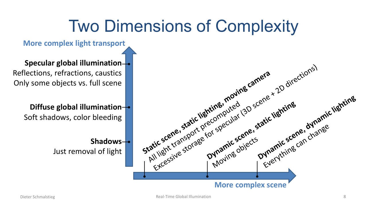
L10_Pg-08: Two axes - light-transport complexity (shadows, diffuse GI, specular GI) and scene dynamics (static scene + moving camera, moving objects, fully dynamic). Each combination admits different precomputation strategies.

Real-time GI has two independent dimensions of difficulty:

Light transport: shadows (removal of light), diffuse GI (soft shadows, colour bleeding), specular GI (reflections, refractions, caustics). Diffuse transport is smooth and compresses well; specular transport has high-frequency directional structure and resists compression.
Scene dynamics: static scene with moving camera (everything can be precomputed, but storage for specular is huge: 3D scene times 2D view direction), dynamic scene with static lighting (objects move, lights and geometry topology fixed), and fully dynamic (everything can change).

The cheapest cell is static scene with diffuse-only transport. The hardest is fully dynamic with specular transport. Different production engines pick different cells of this grid.

Indirect Illumination and Indirect Shadows

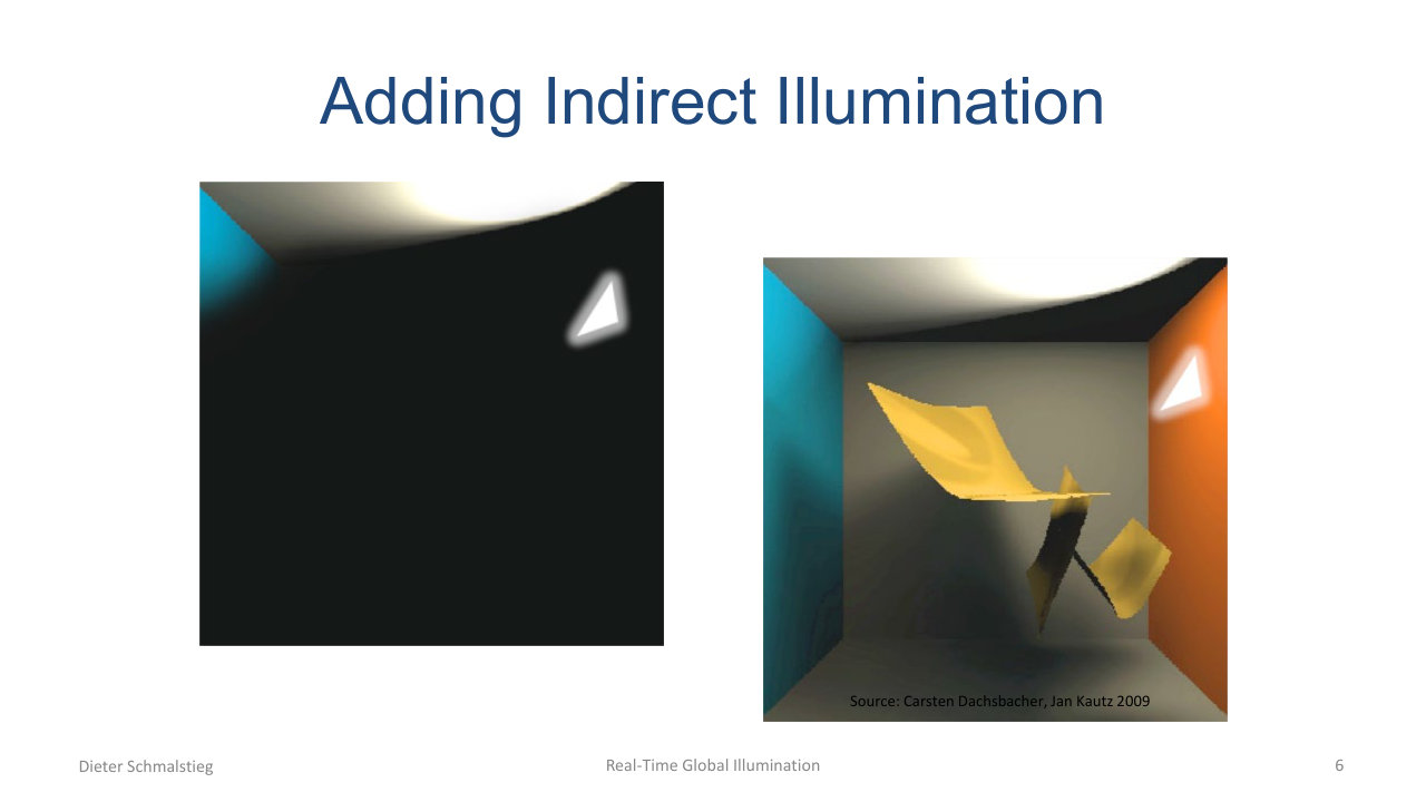
L10_Pg-06: Indirect illumination fills in the dark side of the Cornell box - the yellow rectangles bouncing red and blue tint into the scene.

Direct lighting only is mostly black on surfaces the light cannot see; indirect illumination softens the whole scene and adds colour bleeding from coloured walls. The full effect requires light to bounce at least once off another surface.

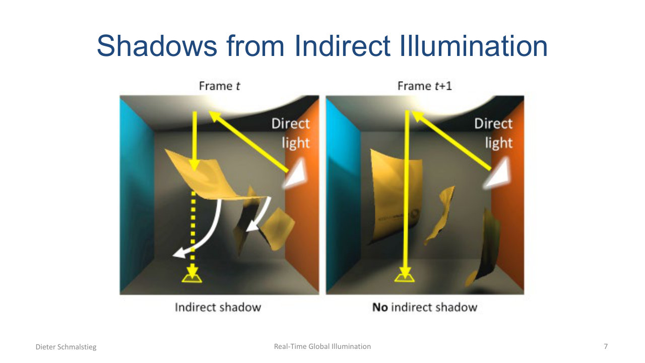
L10_Pg-07: Indirect shadows are non-local - a sheet that occludes the bounced light path between two surfaces casts a shadow that does not match any direct-light shadow.

Indirect shadows are subtle but important: when an occluder breaks the bounced light path between two surfaces, the indirect contribution disappears even though direct lighting is unchanged. Most of the methods in this lecture either approximate or ignore indirect shadows.

3. The Rendering Equation and Its Building Blocks

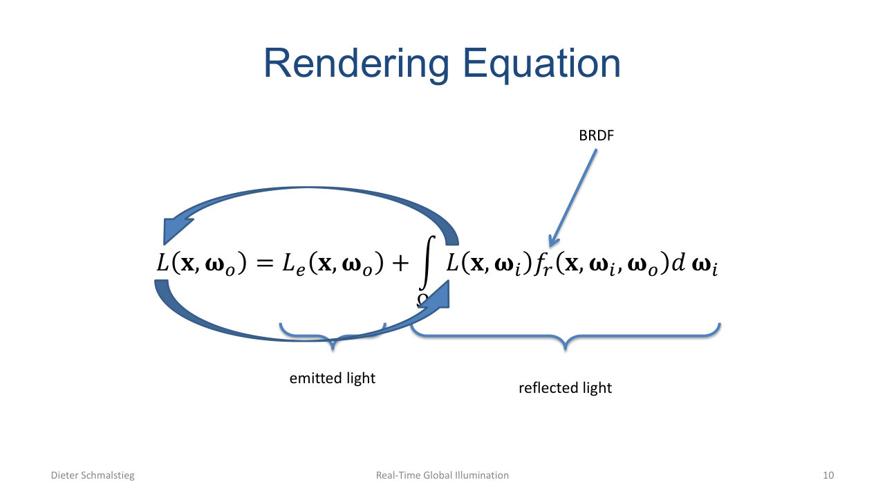
L10_Pg-10: Kajiya's rendering equation - outgoing radiance equals emission plus the integral over the hemisphere of incoming radiance times BRDF.

The reference solution to global illumination is Kajiya’s rendering equation:

$L (x, ω_{o}) = L_{e} (x, ω_{o}) + \int_{Ω} L (x, ω_{i}) f_{r} (x, ω_{i}, ω_{o}) d ω_{i}$

Outgoing radiance at point $x$ in direction $ω_{o}$ equals emitted radiance plus the integral over the hemisphere of incoming radiance weighted by the BRDF. The recursion is in the $L$ on the right-hand side: incoming radiance from direction $ω_{i}$ is itself outgoing radiance from some other surface in the scene.

BRDF

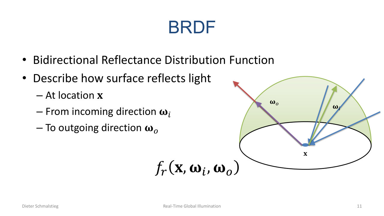
L10_Pg-11: The BRDF $f_r(\mathbf{x}, \boldsymbol{\omega}_i, \boldsymbol{\omega}_o)$ describes how a surface at $\mathbf{x}$ converts incoming light from $\boldsymbol{\omega}_i$ to outgoing light in $\boldsymbol{\omega}_o$.

The BRDF $f_{r}$ is the per-surface function describing reflectance. It obeys three constraints: reciprocity ( $f_{r} (x, ω_{1}, ω_{2}) = f_{r} (x, ω_{2}, ω_{1})$ ), energy conservation ( $\int_{Ω} f_{r} d ω_{i} \leq 1$ ), and positivity ( $f_{r} \geq 0$ ).

Radiance vs. Irradiance

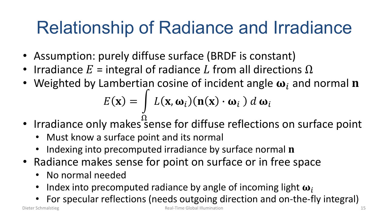
L10_Pg-15: For a purely diffuse surface, irradiance $E(\mathbf{x}) = \int L(\mathbf{x}, \boldsymbol{\omega}_i)(\mathbf{n} \cdot \boldsymbol{\omega}_i) \, d\boldsymbol{\omega}_i$. Irradiance is indexed by surface normal; radiance is indexed by incoming direction.

The two radiometric quantities used throughout the lecture:

Irradiance $E$ is radiant flux per unit area ( $W / m^{2}$ ). It is a scalar with no directional information. For purely diffuse surfaces, $E$ is the cosine-weighted integral of incoming radiance over the hemisphere. It only makes sense at a surface point with a known normal.
Radiance $L$ is radiant flux per unit area per solid angle ( $W / m^{2} \cdot sr$ ). It carries direction, makes sense in free space (no normal needed), and is what you need for specular reflection.

Diffuse caches store irradiance (cheaper, precomputed, indexed by normal). Specular caches store radiance (richer, needs runtime integration).

Neumann Expansion

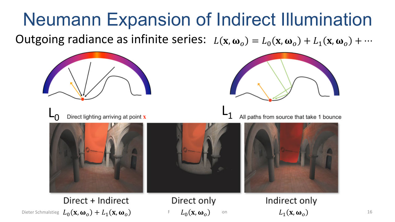
L10_Pg-16: The recursive rendering equation expanded as $L = L_0 + L_1 + \ldots$, with $L_0$ direct lighting and $L_1$ one-bounce indirect. The direct-only image is mostly black; the indirect-only image has all the colour bleeding.

Solving the rendering equation by iteration gives an infinite series $L = L_{0} + L_{1} + L_{2} + \dots$ where $L_{k}$ is the contribution of paths with exactly $k$ bounces. Real-time methods stop at small $k$ (often just $L_{0} + L_{1}$ ). The price is that high-order effects (caustics, multi-bounce colour bleeding) are missing or faked.

4. Path Tracing as Reference

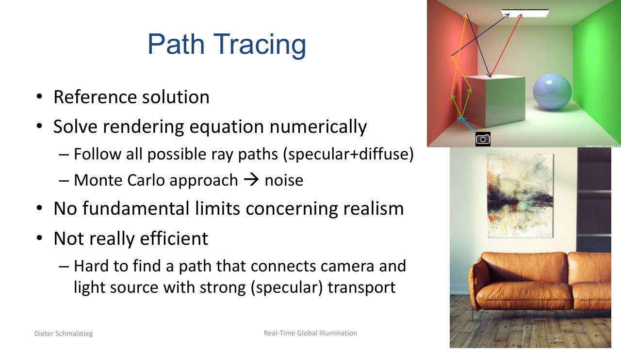
L10_Pg-17: Path tracing follows ray paths between camera and light - the reference solution. Monte Carlo sampling means noisy results that converge to ground truth.

Path tracing solves the rendering equation numerically by Monte Carlo. From the camera, for each pixel, shoot a ray; on hit, generate a new ray in a random direction weighted by the BRDF; continue until the path terminates (Russian roulette) or hits a light source. Average over many paths.

Variants:

Shooting: trace from the light until the camera is hit. Good for caustics, bad for shaded surfaces (most paths waste).
Gathering: trace from the camera until a light is hit. Standard inversion.
Bidirectional path tracing: trace from both ends and connect.

Pros: no fundamental limits on realism, handles every transport type, mathematically straightforward. Cons: noisy, slow, and finding paths that connect camera and light through strong specular transport is hard.

The point of the rest of the lecture is that everything else is a cheap approximation of path tracing.

5. The Real-Time Recipe

For real time, the answer is always the same shape:

Approximate where you can: semi-global (some objects only), low-order (1-2 bounces), ignore specular.
Cache wherever possible: precompute once or rarely.
Prefer rasterisation over ray tracing where the topology fits the GPU.

The general two-pass pattern: pass 1 computes some piece of light transport into a cache; pass 2 rasterises the camera view and reads the cache for indirect lighting. Each pass independently chooses transport type (diffuse or specular), rendering method (raster or ray), and update rate (once, sometimes, or every frame).

Method	Transport	1st pass result	2nd pass
Radiosity	Diffuse	Light maps	Texture mapping
Photon mapping	Diffuse + specular	Photon map	Ray tracing
Instant radiosity	Diffuse	Shadow maps	Deferred rendering
RSM / probes	Diffuse + specular	RSM / probe map	Deferred + sampling

6. Radiosity

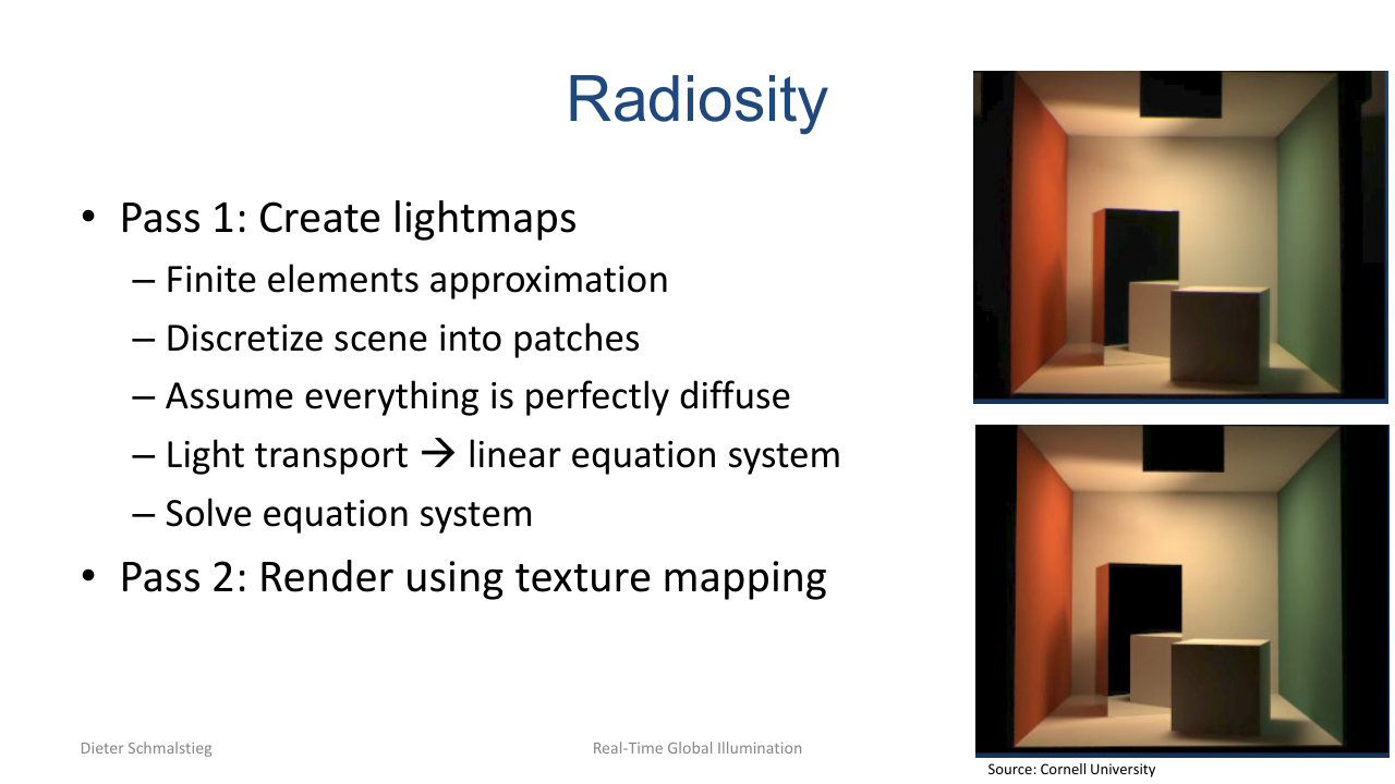
L10_Pg-23: A Cornell-box-style scene rendered with radiosity - soft shadows and red/green colour bleeding from the walls.

Radiosity is the classical finite-element solution for diffuse light transport. Pass 1 builds light maps (textures storing radiosity per surface element). Pass 2 just textures the geometry.

Patches

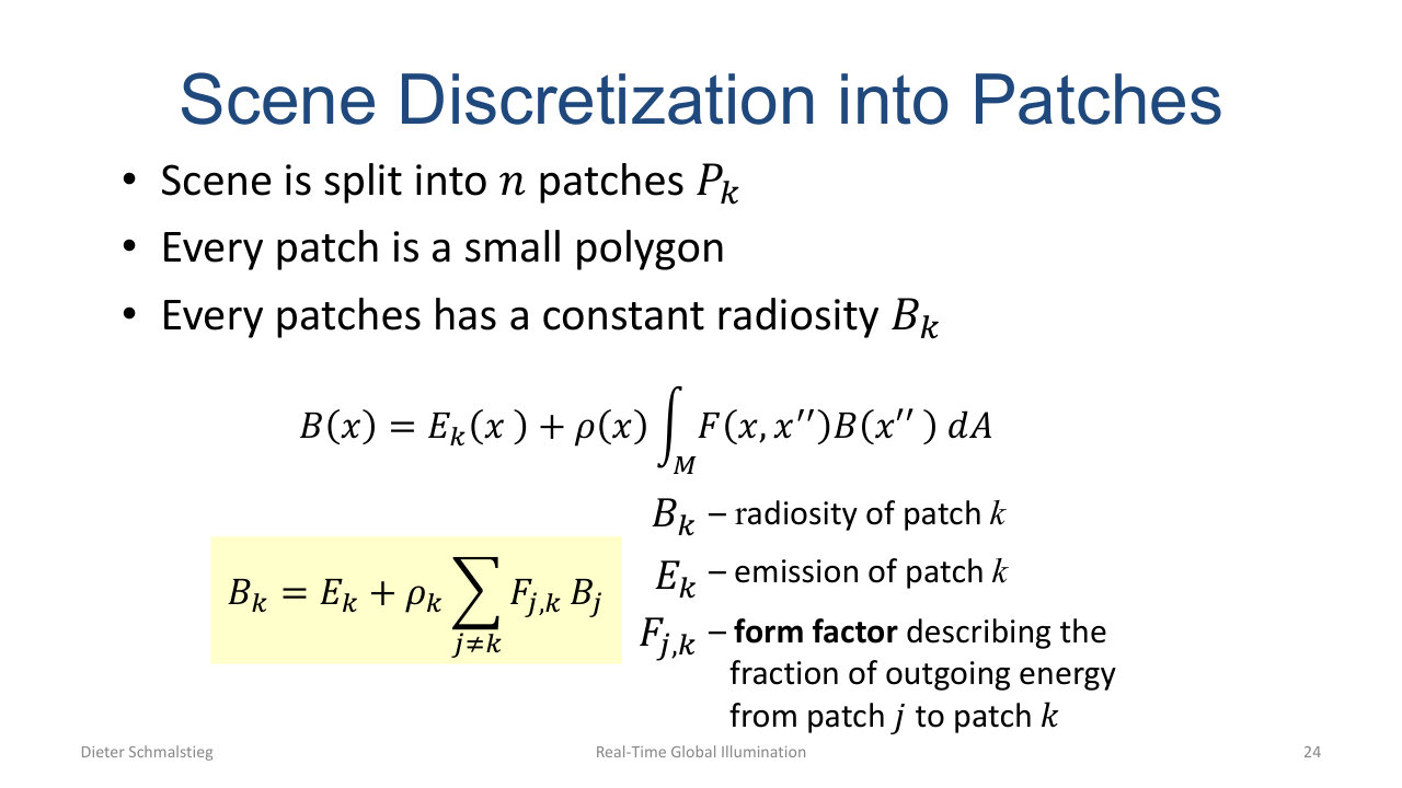
L10_Pg-24: Scene split into $n$ patches $P_k$, each with constant radiosity $B_k$. Discrete radiosity equation: $B_k = E_k + \rho_k \sum_{j \ne k} F_{j,k} B_j$.

Discretise the scene into $n$ patches $P_{k}$ , each treated as a small Lambertian polygon with constant radiosity $B_{k}$ . The discrete radiosity equation is

$B_{k} = E_{k} + ρ_{k} \sum_{j \neq = k} F_{j, k} B_{j}$

where $E_{k}$ is emission, $ρ_{k}$ is reflectance, and $F_{j, k}$ is the form factor, the fraction of energy leaving patch $j$ that arrives at patch $k$ .

Form Factors

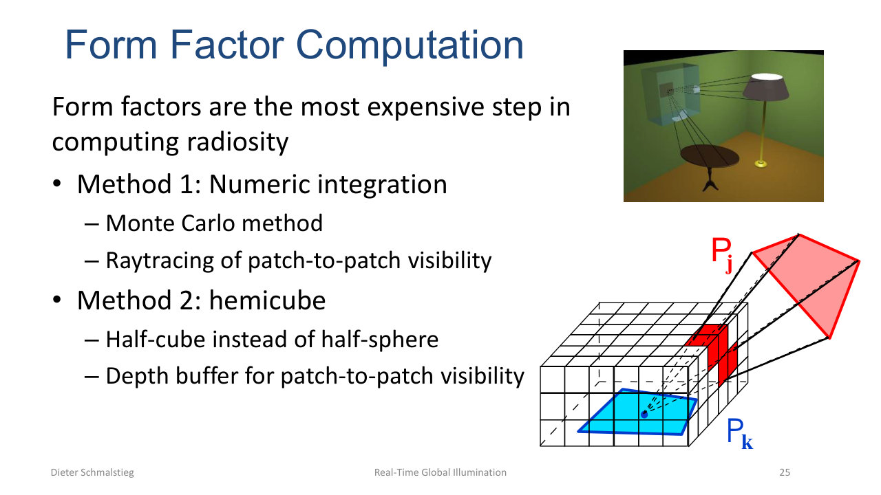
L10_Pg-25: Form factors are computed by numeric integration (Monte Carlo ray tracing) or by the hemicube method - rasterise the scene onto a half-cube around the receiver patch, using the depth buffer for occlusion.

Form factors dominate the cost. Two ways to get them:

Numeric integration: Monte Carlo with patch-to-patch visibility by ray tracing.
Hemicube: use a half-cube around the receiver instead of a half-sphere; rasterise each emitter through its depth buffer for visibility. Each pixel of the cube face contributes to the form factor by its solid angle.

Solving the Linear System

The discrete radiosity equation is an $n \times n$ linear system $(I - ρF) B = E$ . Solve with Gaussian elimination, LU, or Gauss-Seidel iteration. Two complementary iteration views:

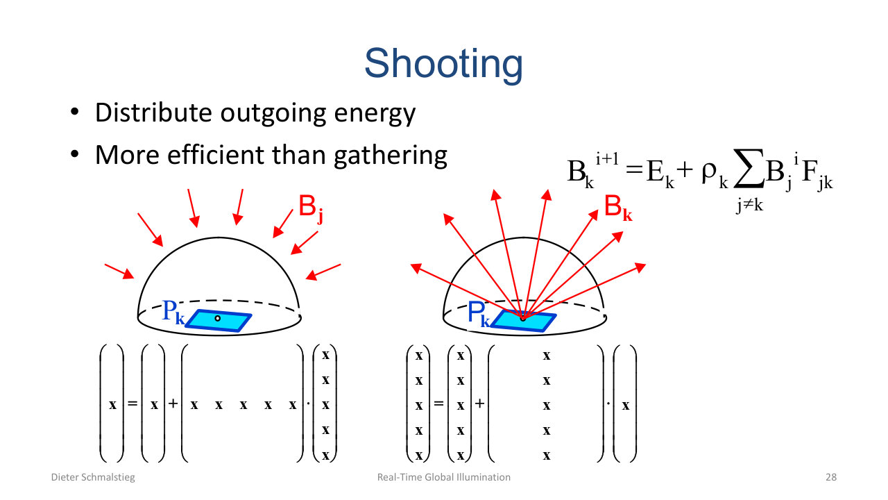
L10_Pg-28: Gathering vs. shooting - gathering collects energy into one patch (one row of the matrix), shooting distributes one patch's energy to all others (one column). Shooting converges faster in practice.

Gathering is the standard Gauss-Seidel: update one patch by summing contributions from all others. Shooting is the reverse: pick the brightest unshot patch, distribute its energy to everyone, then repeat. Shooting converges faster because the brightest patches dominate the result.

Memory and compute are both heavy: $n^{2}$ form factors, large dense matrix, only diffuse transport.

7. Photon Mapping

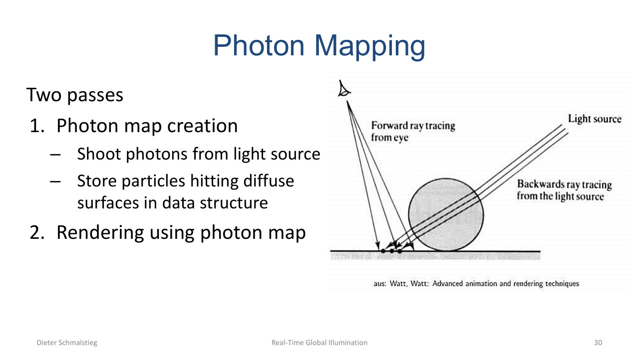
L10_Pg-30: Photon mapping - forward rays from the light source land photons on diffuse surfaces, then backward rays from the camera sample them.

Photon mapping is a two-pass method handling diffuse plus some specular transport, including caustics.

Pass 1: photon map creation. Shoot photons from the light source through the scene. At each diffuse hit, store the photon in a spatial data structure (typically a kd-tree). Russian roulette terminates paths probabilistically.

Pass 2: rendering. Backward ray tracing from the camera. At each visible surface point, sample the photon map: collect photons within radius $r$ of the point; the number of photons equals the local intensity.

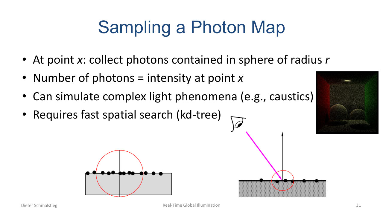
L10_Pg-31: At point $x$, count photons within sphere of radius $r$. The kd-tree makes this lookup fast. Caustic patterns emerge naturally because photons cluster where specular paths converge.

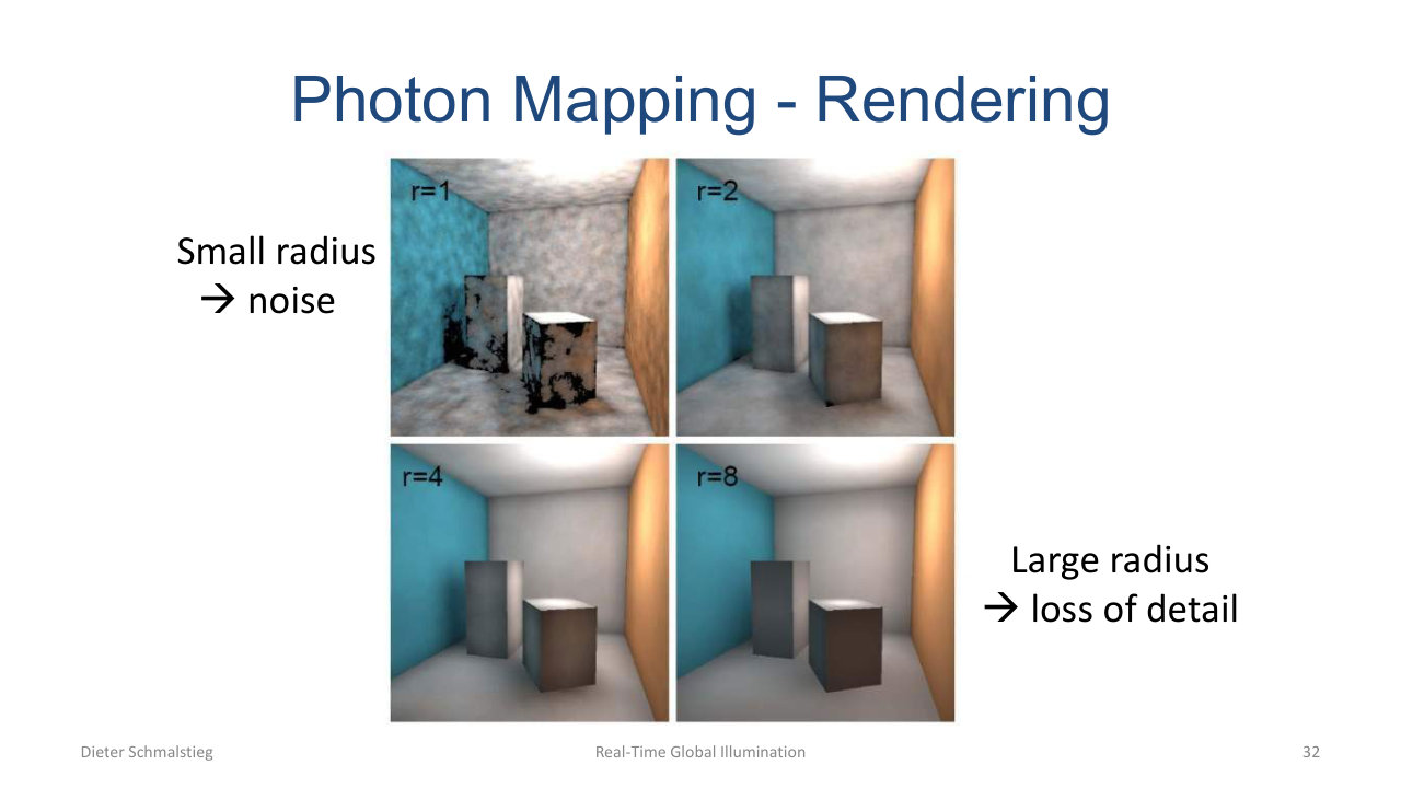
L10_Pg-32: The radius $r$ trades noise for blur - $r = 1$ is grainy, $r = 8$ is smooth but loses detail.

The radius $r$ is the central knob: small $r$ gives noisy, sparse coverage; large $r$ smooths the result but blurs sharp features (the corner of a caustic). Production photon mappers use adaptive radii.

8. Caching Frameworks

Every method in this lecture is some form of render cache. The cache is indexed by some combination of position and orientation, and stores either radiance or irradiance.

Indexing	Examples	Comment
Position only (3D)	Photon maps (kd-tree), radiosity patches	Surface positions or volumetric points
Orientation only (2D)	Environment maps (cubemap)	Direction without position; assumes infinitely distant env
Projective space (2.5D)	Shadow maps, instant radiosity	3D points indexed via 2D depth map
Position + orientation (5D)	Irradiance volumes, light propagation volumes, probes	Position as main index, orientation as sub-index

Cubemaps, Paraboloids, Octahedral Maps

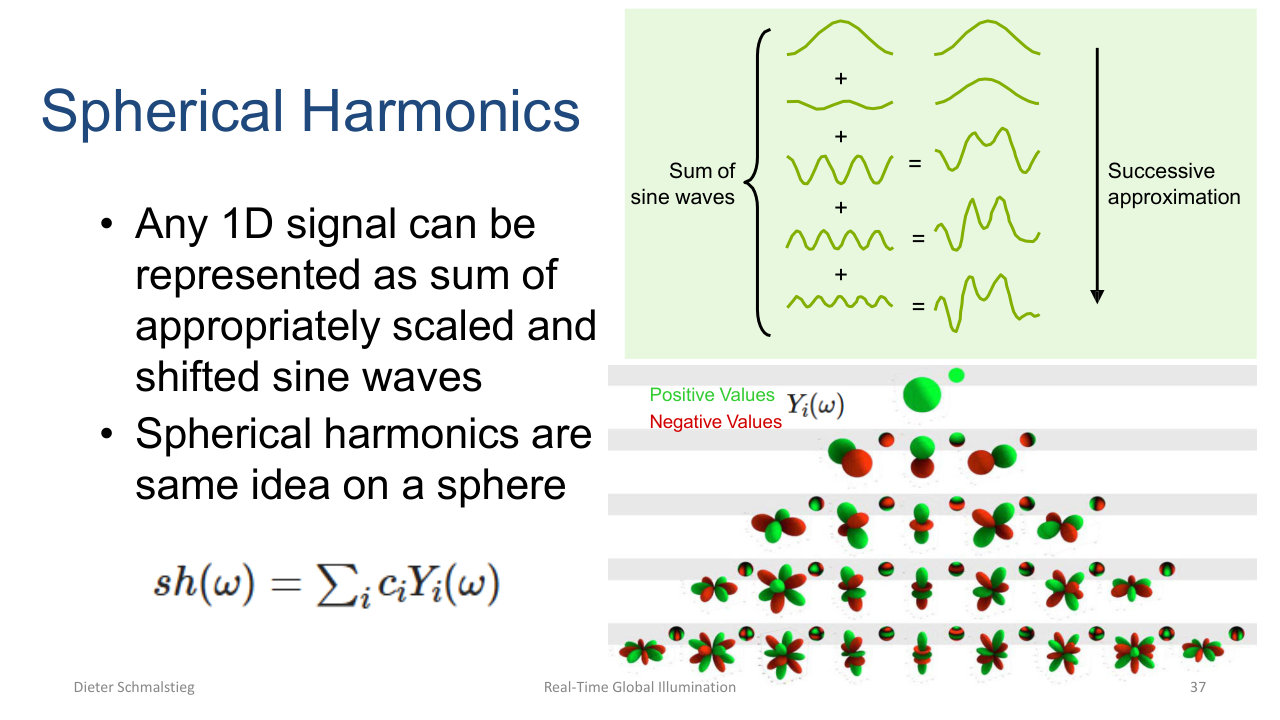
L10_Pg-37: Spherical harmonics - decompose a function on a sphere into a sum of basis functions (analogue of Fourier series on a 1D interval). Successive approximation by truncating the series.

The standard 2D parametrisations of orientation are cubemap, dual paraboloid map, octahedral map, and spherical harmonics (SH). The first three are texture-based; SH is a sum-of-basis-functions decomposition like Fourier series for the sphere.

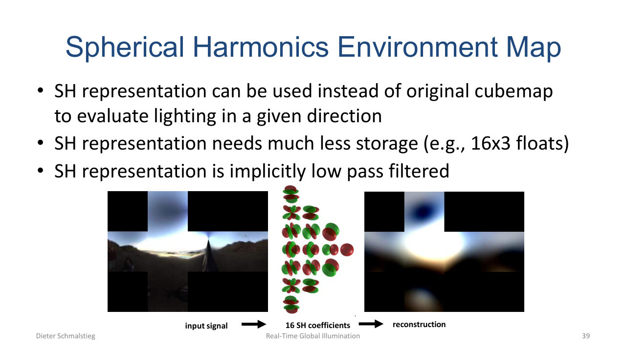
L10_Pg-39: 16 spherical-harmonic coefficients reconstruct a low-pass version of a cubemap environment. SH gives compact storage (16 floats per colour channel) but only diffuse-quality detail.

SH is heavily used for diffuse environment lighting: 16 SH coefficients (4 bands) per colour channel is about 48 floats, enough for smooth diffuse environment lighting. SH is intrinsically low-pass, so it cannot represent sharp specular highlights.

9. Instant Radiosity and Virtual Point Lights

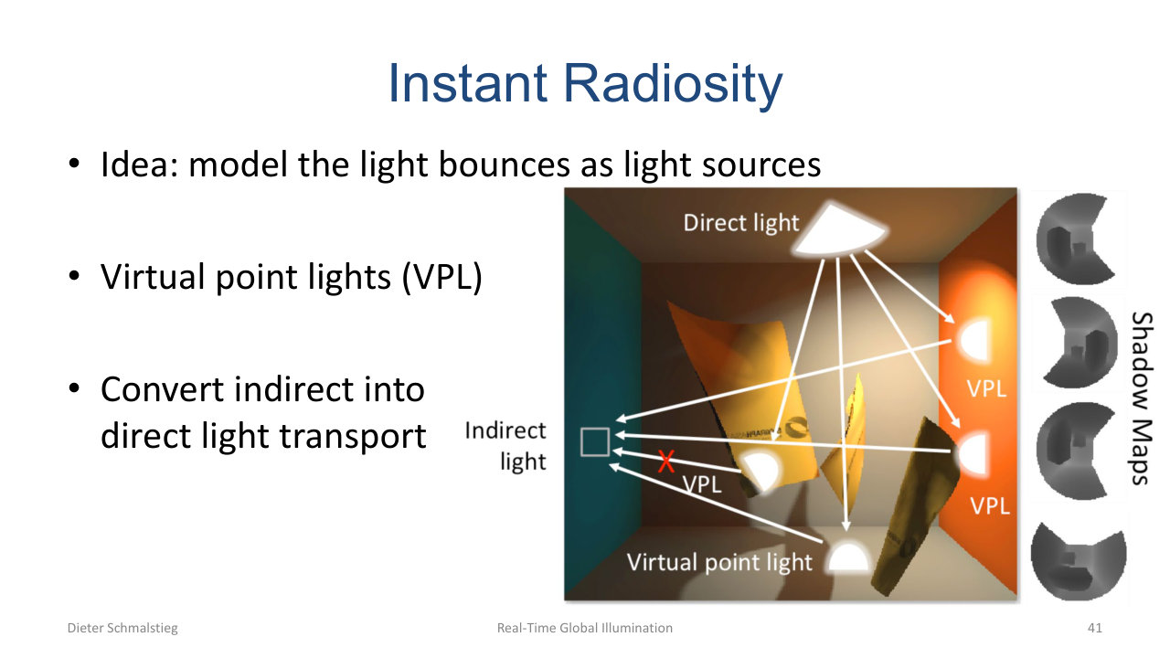
L10_Pg-41: Instant radiosity converts indirect lighting into direct lighting from many virtual point lights (VPLs) scattered through the scene.

The instant-radiosity trick: replace indirect bounces by a swarm of virtual point lights (VPLs) placed at the photon hit points. Indirect lighting then reduces to many direct lights, which the renderer already knows how to handle.

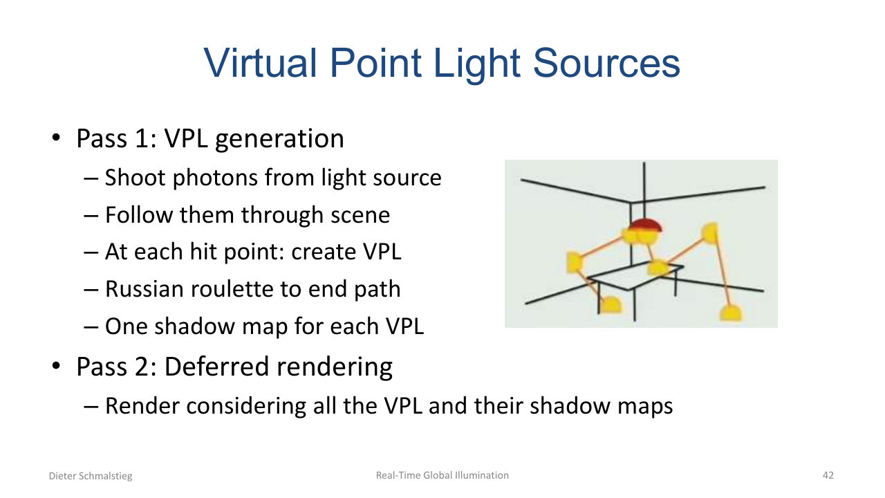
L10_Pg-42: Pass 1 shoots photons from the light, creates a VPL at each hit, generates a shadow map per VPL. Pass 2 does deferred rendering using all VPLs and their shadow maps.

Pass 1: shoot photons; at each hit point spawn a VPL; render a shadow map for each VPL.

Pass 2: deferred rendering accumulating contributions from all VPLs and their shadow maps.

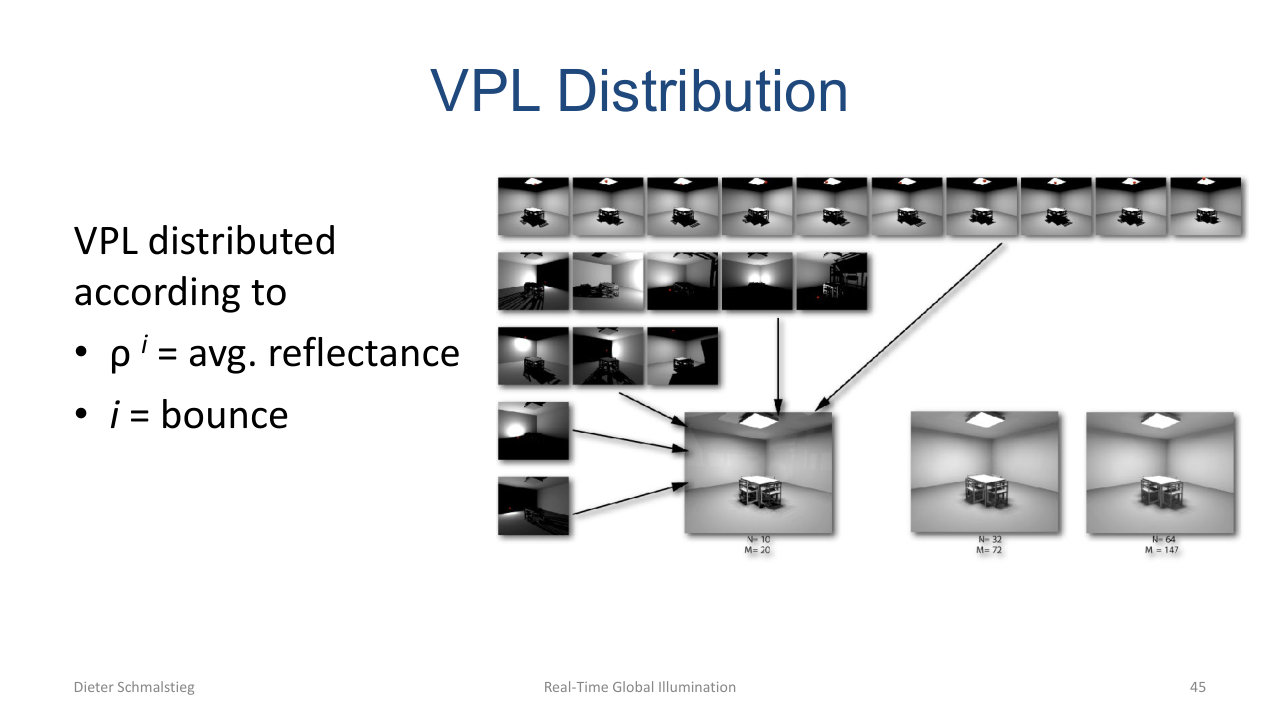
L10_Pg-45: VPL distribution as photons cascade through the scene - weight $\rho^i$ falls off geometrically with bounce $i$.

VPLs are distributed according to the local reflectance $ρ^{i}$ raised to the bounce index $i$ : bounce-1 VPLs dominate, bounce-2 contribute less, etc.

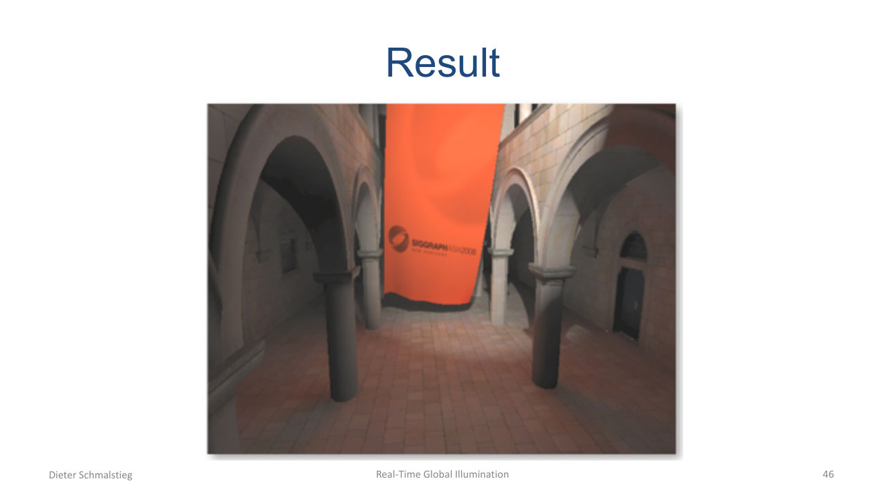
L10_Pg-46: Sponza atrium lit by instant radiosity - warm bounced light fills the arcades.

Problem: Too Many Shadow Maps

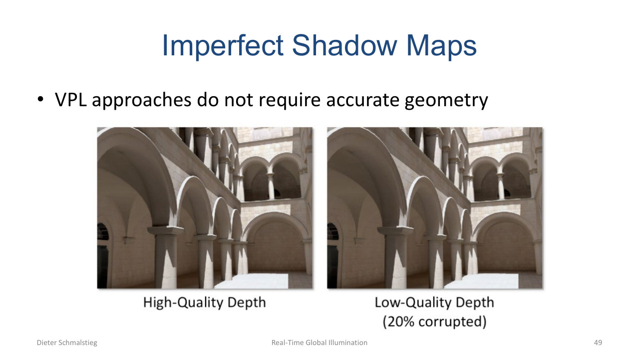
L10_Pg-49: Imperfect shadow maps - VPL shadow maps do not need accurate geometry. Even 20% corrupted depth gives a result close to high-quality.

1024 VPLs times a 100K-triangle scene means 100M triangles to rasterise just for shadow maps. The optimisation insight is that VPL contributions are individually weak and noisy, so each VPL’s shadow map can be very low-quality without visible degradation. This is Imperfect Shadow Maps (ISM).

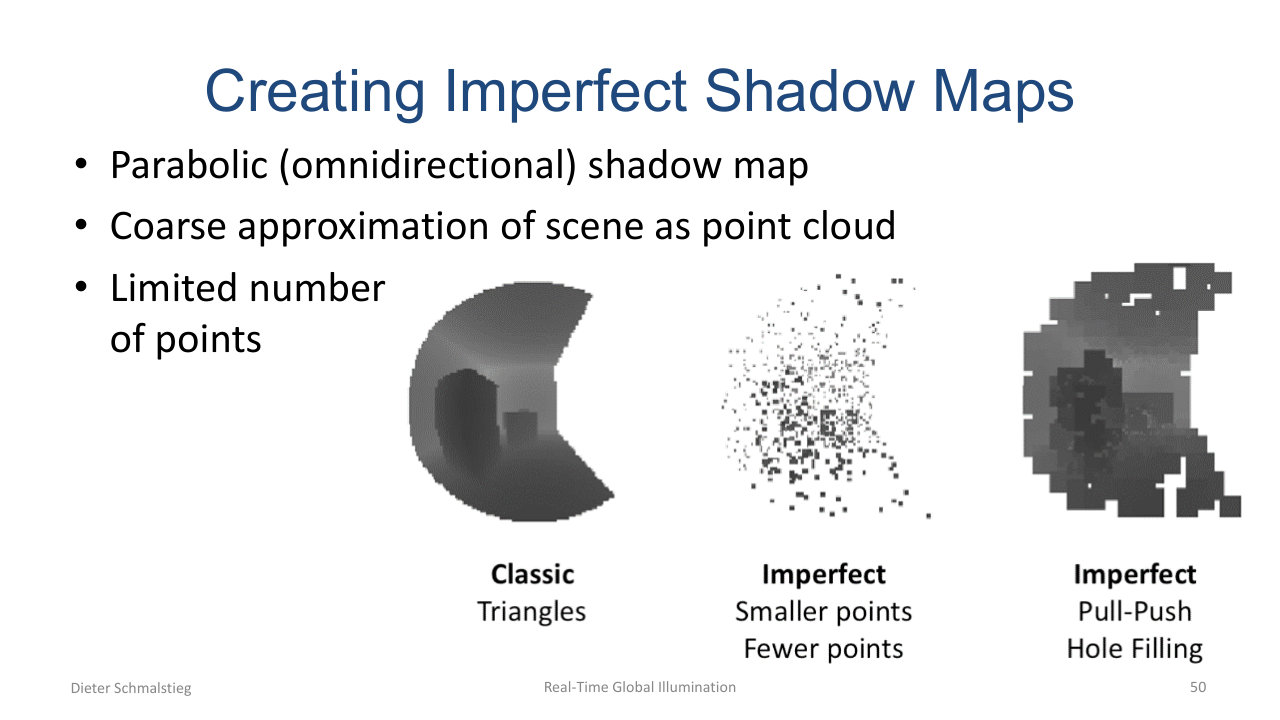
L10_Pg-50: ISM substitutes triangles with a coarse point cloud per VPL, then fills holes with pull-push interpolation.

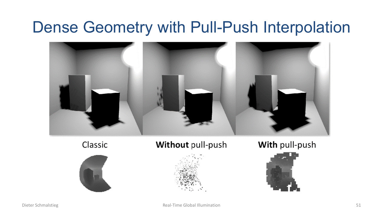
L10_Pg-51: Pull-push interpolation on a sparse point-cloud shadow map turns a noisy depth into a usable one.

ISM approximates the scene as a coarse point cloud, rasterises it into a parabolic (omnidirectional) shadow map per VPL, then fills holes with a pull-push filter.

Interleaved Sampling

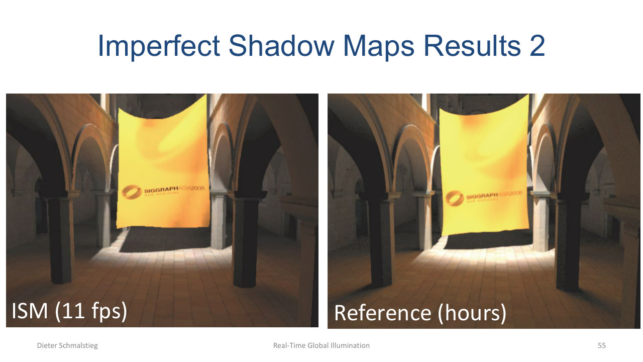
L10_Pg-55: ISM at 11 fps next to a hours-long reference path-traced image - the difference is small enough to ship.

To reduce shading cost, each pixel uses only a random subset of VPLs (interleaved sampling), and the result is denoised with an edge-aware bilateral filter. Combined with ISM, instant radiosity can hit interactive frame rates on Sponza-scale scenes.

10. Reflective Shadow Maps

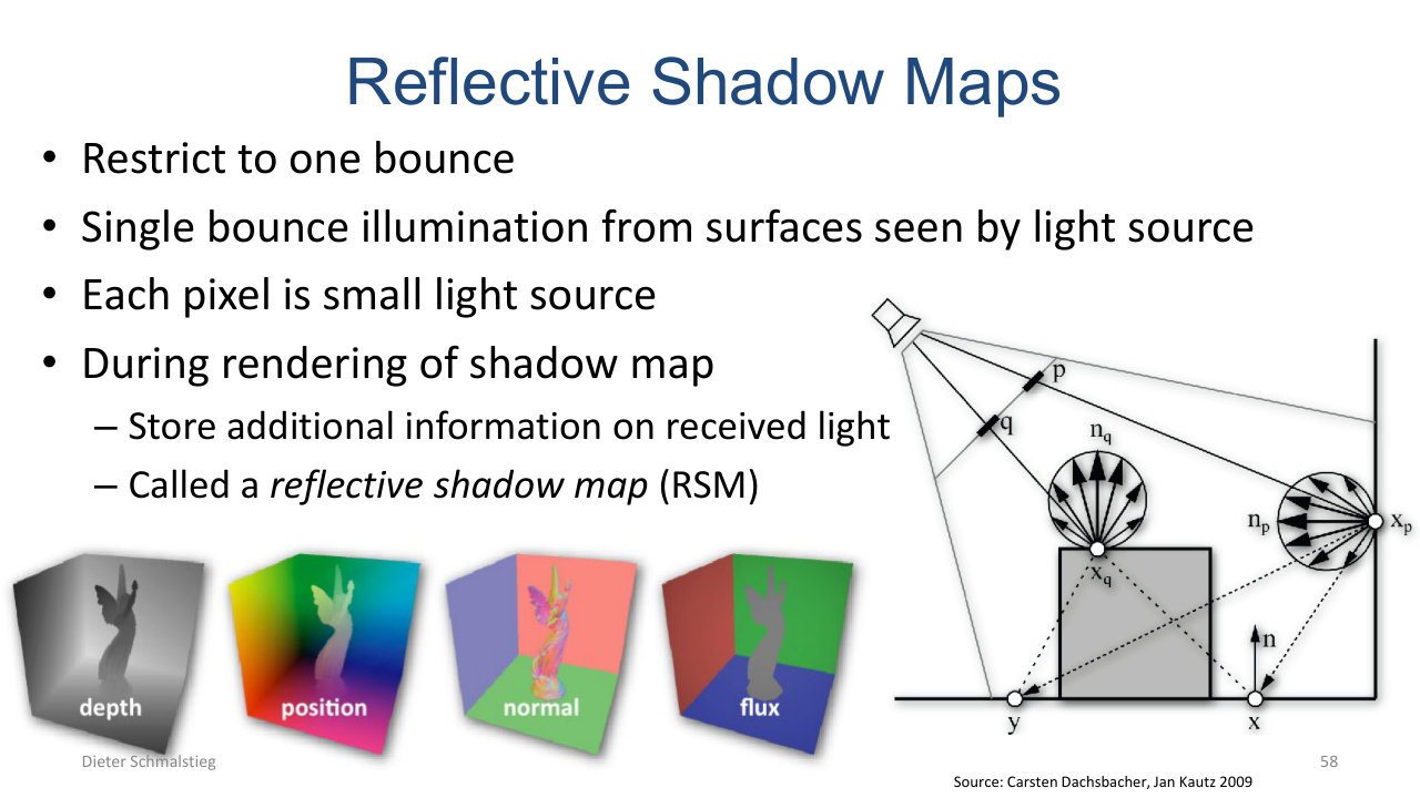
L10_Pg-58: A reflective shadow map (RSM) is a shadow map that also stores position, normal, and outgoing flux per pixel - each pixel becomes a small VPL.

A reflective shadow map restricts indirect lighting to one bounce from surfaces visible to the light source. Each pixel of the light’s shadow map stores not just depth, but also position, normal, and flux. The shadow map becomes a flat array of VPLs, automatically distributed where the light hits.

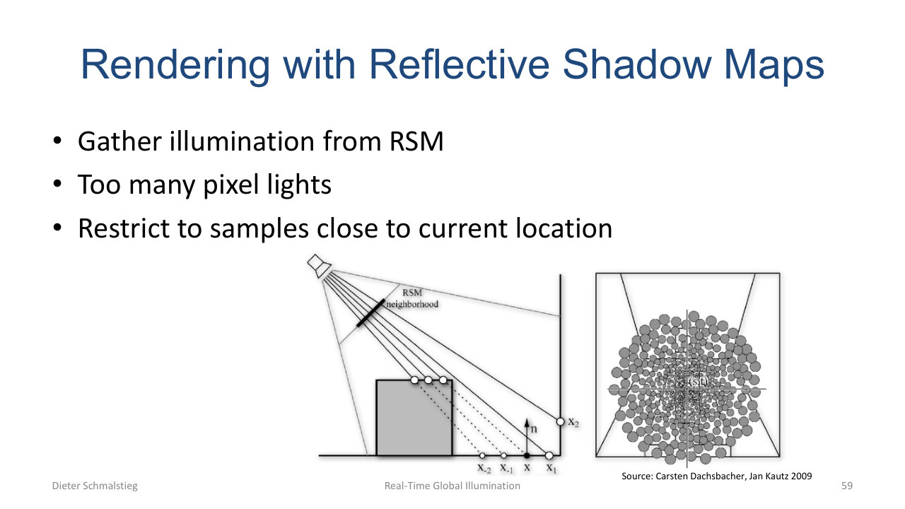
L10_Pg-59: Gather illumination from RSM. Too many RSM pixels to sample all of them, so restrict to samples close to the current pixel's projection into the RSM.

For each visible surface point, gather illumination from RSM pixels close to that point’s projection in light space. Sampling density falls off with distance, motivated by the assumption that distant RSM pixels contribute weakly to the local bounce.

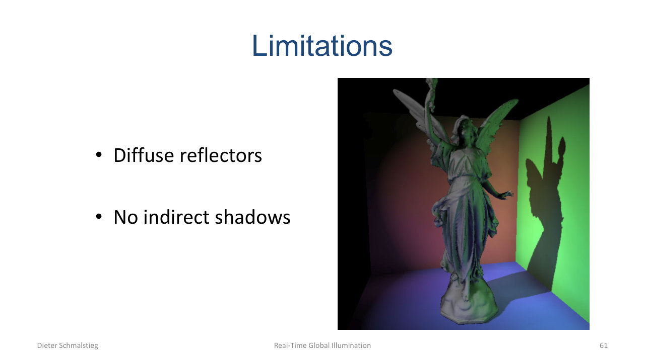
L10_Pg-61: RSM limitations - diffuse reflectors only, and the result has no indirect shadows (the cast shadow on the right wall is wrong).

Limitations: only diffuse reflectors, and no indirect shadows (RSM does not know about geometry between the bounce point and the receiver). Most cheap real-time GI in the 2010s built on this scheme.

11. Illumination Probes

The modern dominant approach in production engines (Unity, Far Cry, Unreal). Probes are points in space where directional incoming light has been precomputed.

Store irradiance for diffuse reflection (cheap, normal-indexed, but only diffuse).
Store radiance for specular reflection (richer, requires runtime BRDF integration).
Place probes on a world-space grid, on an artist-chosen list, or in screen space.
Use the closest probe (or interpolate several) when shading a surface point.

Octahedral Representation

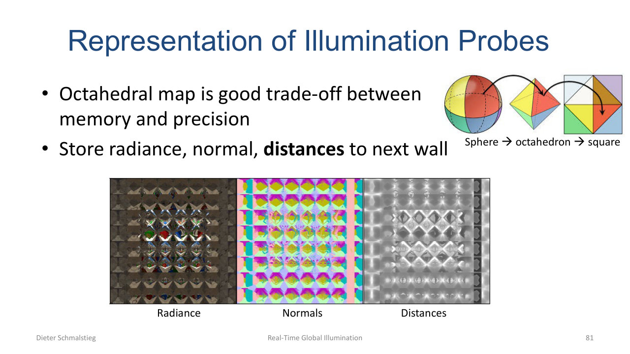
L10_Pg-81: An illumination probe stored as octahedral map of radiance, normals, and distances per direction. Octahedral mapping unfolds a sphere into a square with low distortion.

Octahedral maps are the production-friendly parametrisation: unfold the sphere through an octahedron into a square texture. Each texel stores radiance, surface normal, and distance to the nearest occluder in that direction. The distance map is what makes leak-free indirect light possible.

Ray Tracing the Probe

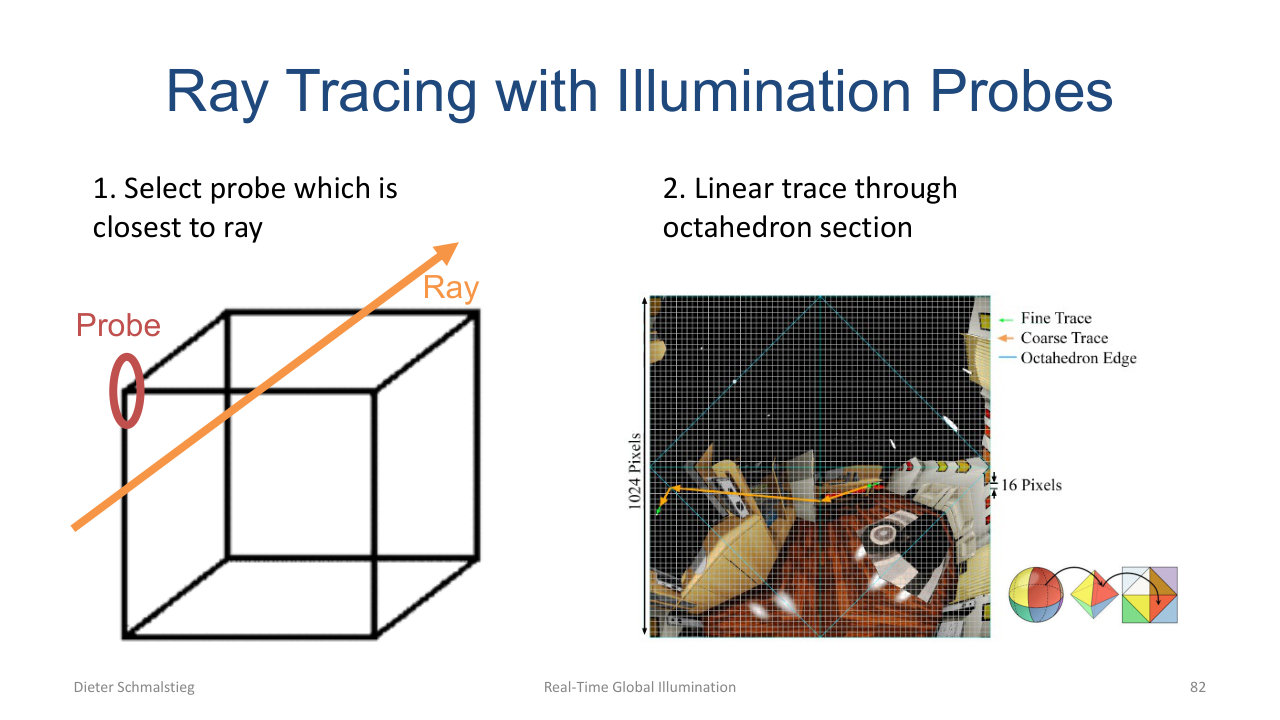
L10_Pg-82: Trace a ray against the probe by picking the closest probe to the ray and linearly tracing through the octahedron section the ray covers.

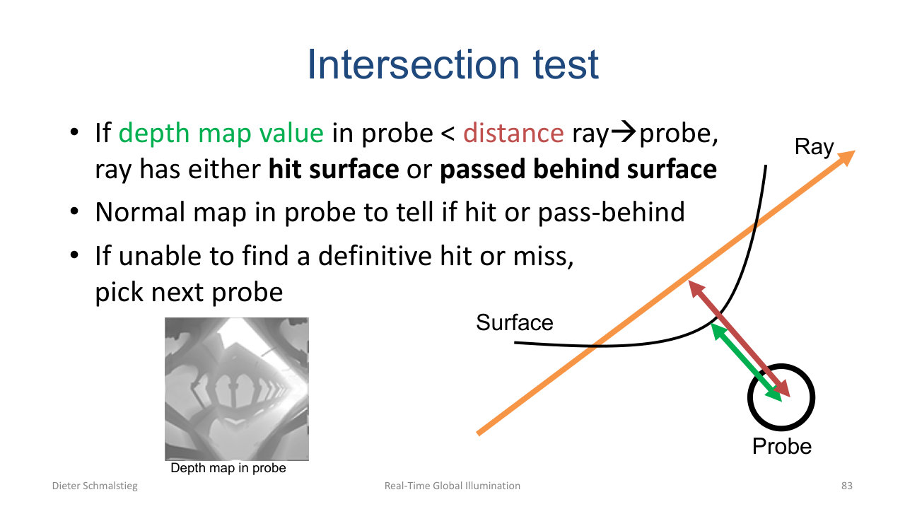
L10_Pg-83: Intersection test - if the probe's depth map value is less than the distance from ray origin to probe, the ray has either hit the surface or passed behind it. The normal map disambiguates.

The intersection test compares the ray-to-probe distance against the depth map stored in the probe. The normal map distinguishes a true hit from a pass-behind.

Light Leaks

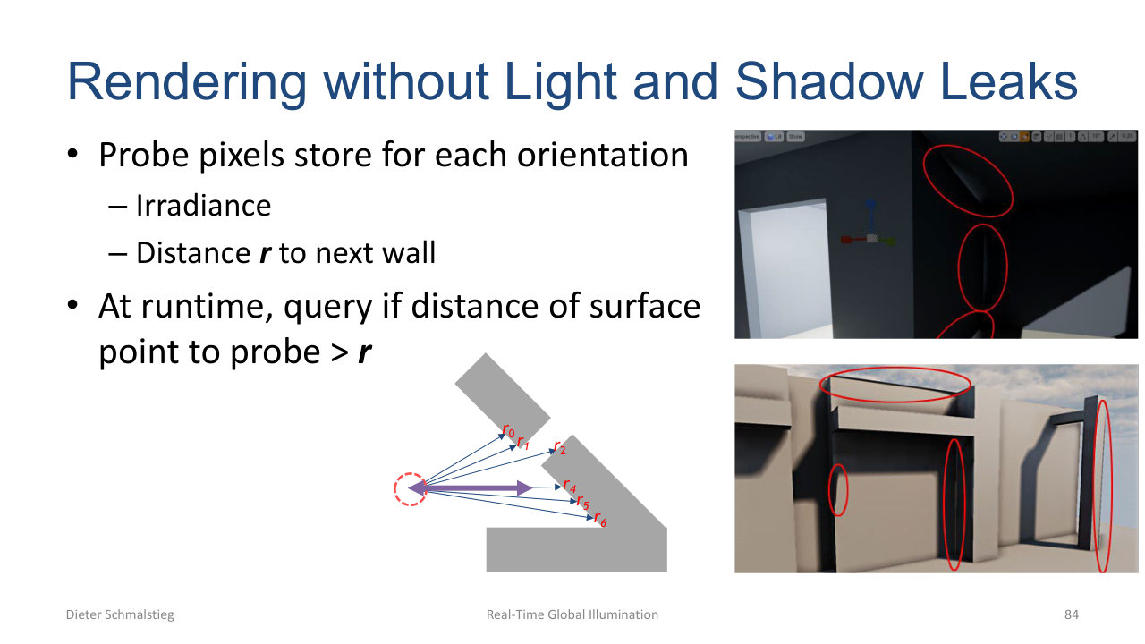
L10_Pg-84: Light leaks happen when the receiver is on the wrong side of a wall relative to the probe. Using per-direction distance $r$ stored in the probe, reject the contribution if the distance from surface to probe exceeds $r$.

The classic failure mode: a probe placed near a wall contributes light through the wall to a receiver behind it. The cure is the distance map. At runtime, for each direction towards the probe, check that the distance from the surface point to the probe is less than the recorded distance to occluder; if not, the contribution is rejected.

Why Interpolation Is Mandatory

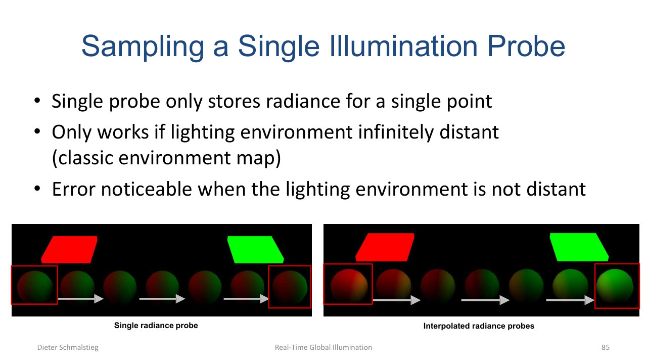
L10_Pg-85: A single radiance probe assumes infinitely distant lighting. When the lighting environment is nearby (red and green panels), the single-probe approximation goes flat; interpolating between multiple probes recovers the gradient.

A single probe only works if the lighting environment is infinitely distant. For nearby lighting (the red and green panels of a Cornell box), the result is flat and wrong. Interpolation between several probes restores the gradient.

Screen-Space Probes

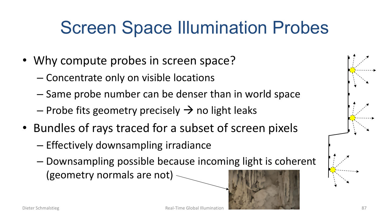
L10_Pg-87: Screen-space probes concentrate samples on visible pixels, hugging geometry precisely so they cannot leak.

Screen-space probes are placed only at visible pixels, giving denser coverage than the same number of world-space probes and avoiding leaks because the probe is always on the surface. They effectively downsample incoming irradiance, which is acceptable because incoming light is much smoother than the normal field, so a low-resolution probe grid can still produce a high-resolution shaded image.

Hybrid Caching

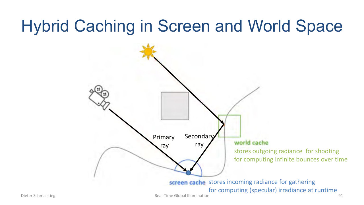
L10_Pg-91: Hybrid caching - world-space probes store outgoing radiance for shooting (capture infinite bounces over time), screen-space probes store incoming radiance for gathering (compute irradiance at the current pixel).

Lumen-style engines combine both: world-space probes are slowly updated and feed shooting (each world probe scatters light into neighbour probes, accumulating infinite bounces); screen-space probes are updated per frame and gather incoming radiance for shading.

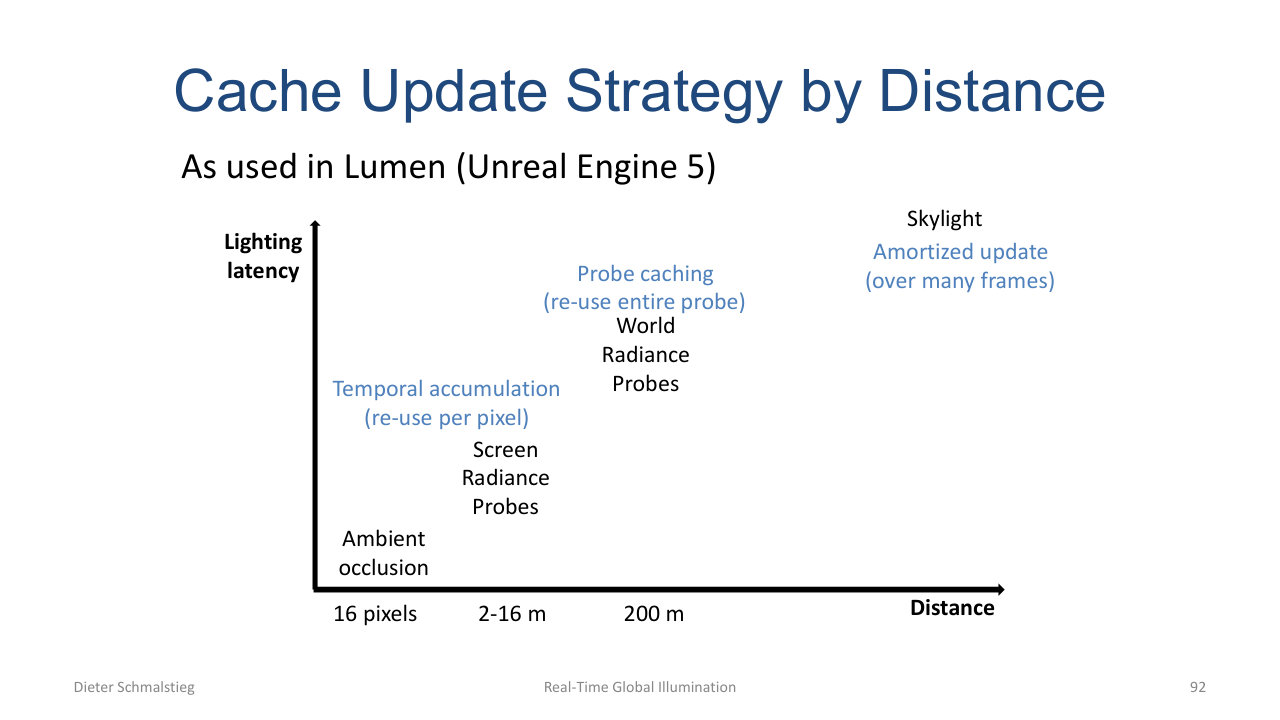
L10_Pg-92: Cache update strategy by distance (Lumen) - ambient occlusion under 16 pixels updates per pixel, screen-space probes (2-16 m) use temporal accumulation, world probes (~200 m) use probe-level caching, skylight is amortised over many frames. Lighting latency grows with distance because the eye is less sensitive there.

The cache update strategy is the engineering payoff: different cache levels are updated at different rates, with lighting latency allowed to grow with distance from the camera.

12. Precomputed Radiance Transfer

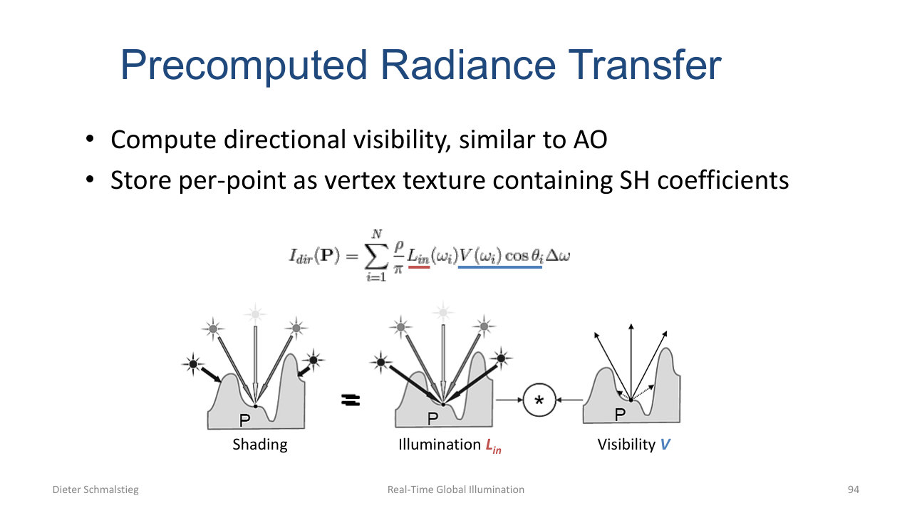
L10_Pg-94: PRT factors shading into illumination $L_{in}$ (the environment light) and visibility $V$ (precomputed directional transfer at each surface point). Final shading is the dot product of two SH vectors.

PRT addresses a subtle remaining problem: probes do not know about self-occlusion and bounced light within the same object. The visibility integral inside a teapot’s handle requires per-vertex precomputed information.

PRT factorises the rendering at point $P$ as

$I_{d i r} (P) = \sum_{i = 1}^{N} \frac{ρ}{π} L_{in} (ω_{i}) V (ω_{i}) cos θ_{i} Δ ω$

The light source $L_{in}$ is independent of the geometry. The directional visibility function $V$ (cosine-weighted, including self-occlusion and bounces inside the object) is independent of the lighting.

Precompute $V$ offline via ray tracing and store it per vertex as SH coefficients. At runtime, evaluate the environment lighting $L_{in}$ as SH coefficients too. Diffuse shading is then a dot product of two SH vectors per vertex.

The price is that the precomputation is per-object and per-pose, so PRT works best for static geometry under dynamic environment lighting.

💡 Intuition

Every method in this lecture is the same question with a different answer: what part of the rendering equation can I precompute and look up later, and where is the cache allowed to be stale? Radiosity says diffuse irradiance everywhere, no specular ever. Photon mapping says photons in 3D, queried at render time. Instant radiosity says shadow maps for VPLs, possibly imperfect. RSMs say one-bounce light from the shadow map. Probes say sparse 5D cache (position plus direction) interpolated for smoothness. PRT says per-vertex directional transfer cached as SH. The art is choosing which axis (position, direction, time) to coarsen, and trusting that the human visual system will not notice.

🧠 Deep Dive

Three threads run through the lecture.

First, diffuse versus specular asymmetry. Diffuse transport is smooth, compresses into a handful of SH coefficients, can be indexed by normal alone, and tolerates spatial interpolation. Specular transport has high-frequency directional structure that does not compress, must be integrated at runtime, and tolerates almost no spatial blur. Every cache decision (irradiance vs. radiance, SH vs. cubemap, single vs. interpolated probes) is shaped by this asymmetry.

Second, the topology of the cache. Radiosity caches in surface space (light maps indexed by uv). Photon maps cache in 3D position space (kd-tree). RSMs cache in light-projective space (2.5D). World probes cache on a 5D grid (position plus orientation). Screen probes cache on a 2.5D screen-space grid that automatically tracks visibility. Each topology trades storage for query cost, leak resistance, and update rate.

Third, the temporal budget. Truly real-time methods (RSM, screen probes) can afford only per-pixel temporal accumulation. World probes can amortise over many frames if the scene is semi-static. PRT and radiosity precompute offline and ship the result with the scene. Lumen’s tiered cache is what happens when you take this seriously and split lighting latency by distance: nearby light updates fast, far light updates slowly, and the user does not notice because they are looking at nearby light.

The arc of the field is from physically-motivated reference methods (path tracing, photon mapping, radiosity) towards engineered cache hierarchies (Lumen) that abandon physical exactness for frame budget. The exam-relevant point is that knowing what each method gives up is more important than memorising the equations.

Applied Exam Focus

Two-pass GI is a cache: pass 1 builds it, pass 2 reads it. Every method differs only in what is cached, where, and how often it refreshes.
Diffuse transport: store irradiance, index by surface normal, allow spatial interpolation, compress with SH. Specular transport: store radiance, integrate at runtime over BRDF, no spatial blur.
Radiosity: discretise into patches, solve $B = E + ρF B$ linear system, form factors by Monte Carlo or hemicube. Diffuse only. Shooting converges faster than gathering.
Photon mapping: shoot photons, store in kd-tree on diffuse hits, query by radius $r$ . Radius trades noise vs. detail. Handles caustics.
Instant radiosity: replace bounces with VPLs each rendered as a shadow-mapped direct light. Imperfect shadow maps reduce cost by approximating scene as point cloud per VPL plus pull-push.
Reflective shadow maps: one-bounce indirect from light-visible surfaces; each shadow-map pixel is a VPL with position, normal, flux. No indirect shadows.
Illumination probes: sparse 5D cache of incoming light (irradiance for diffuse, radiance for specular). Octahedral parametrisation with per-direction distance avoids leaks. Always interpolate.
Screen-space probes: per-pixel, no leaks, denser than world space, but only see what is visible on screen. Combine with world probes for full coverage.
PRT: factor lighting into environment SH times per-vertex transfer SH. Dot product per vertex per frame. Handles self-occlusion and within-object bounces.
Lumen-style hybrid: different cache levels update at different rates; lighting latency grows with distance.

Self-Check

Why do we distinguish irradiance from radiance in the design of an illumination cache?

Answer

Irradiance is the cosine-weighted integral of incoming radiance over the hemisphere, indexed by surface normal, and only makes sense at a surface point. Radiance is per direction per solid angle, has no normal dependence, and is needed wherever the BRDF is not pure diffuse. A diffuse cache can store irradiance directly and look it up by normal in one tap, which is much cheaper than evaluating a hemispherical integral at runtime. A specular cache must store radiance because the BRDF concentrates the integration around the reflection direction and the outgoing direction is needed at runtime. The choice between caches is therefore really a choice about what kind of reflectance the method supports.

Walk through the radiosity discrete equation $B_{k} = E_{k} + ρ_{k} \sum_{j \neq = k} F_{j, k} B_{j}$ and explain what dominates its cost.

Answer

Patches $P_{k}$ each have constant radiosity $B_{k}$ , emission $E_{k}$ , and reflectance $ρ_{k}$ . The form factor $F_{j, k}$ is the fraction of energy leaving patch $j$ that reaches patch $k$ . Solving the resulting $n \times n$ linear system is one cost, dominated by Gauss-Seidel iterations. The much heavier cost is computing the $O (n^{2})$ form factors themselves, each of which requires either Monte Carlo ray tracing of patch-to-patch visibility or a hemicube rasterisation around the receiver. For real scenes with $n$ in the millions, this is impractical, which is why radiosity has been displaced by VPL- and probe-based methods that compute light transport on the fly.

Why does the photon-mapping radius $r$ trade off noise and blur?

Answer

At a shading point, the renderer sums photons within distance $r$ and treats that count as a local intensity. If $r$ is small, only a few photons land in the sphere and shot-noise dominates (visible as a grainy speckle pattern). If $r$ is large, many photons average in and the result is smooth, but a sharp caustic edge or a sharp colour-bleed boundary gets blurred over the radius because photons from both sides of the edge contribute equally. The radius is a kernel width: too narrow leaks variance, too wide leaks bias. Production photon mappers adapt $r$ based on local photon density.

Why does instant radiosity scale so badly without imperfect shadow maps, and what does ISM exploit?

Answer

Each VPL needs a shadow map; 1024 VPLs over a 100K-triangle scene means rasterising 100M triangles just for shadow maps, before any shading. ISM exploits the fact that each VPL contributes a small, smoothed fraction of the final shading, so its shadow map can be very low quality without visible artefacts. ISM approximates the scene as a coarse point cloud per VPL, rasterises that point cloud into a parabolic shadow map, and fills holes with pull-push interpolation. Combined with interleaved sampling (each pixel uses only a random subset of VPLs, denoised with a bilateral filter), instant radiosity becomes interactive even on Sponza-scale scenes.

Reflective shadow maps and illumination probes both cache indirect light. What does each capture and what does each miss?

Answer

An RSM is a shadow map augmented with position, normal, and flux per pixel; it captures exactly the surfaces visible from the light source after one bounce. It misses higher bounces, anything not visible to the light, and indirect shadows. Illumination probes capture incoming light at sparse points in space, integrated over the hemisphere; they capture multi-bounce light if the probe pipeline shoots from one probe to its neighbours, and handle dynamic occluders via the per-direction distance map. Probes miss self-occlusion within an object and bounced light inside an object (which is what PRT covers), and they are blurry compared to RSM’s per-pixel one-bounce result.

Why do illumination probes need a per-direction distance map, and how does it prevent light leaks?

Answer

A probe records incoming light at one point in space, but a shaded surface can be on either side of an occluder relative to that probe. Without extra information, light from beyond the wall leaks through. The distance map stores, for each outgoing direction from the probe, the distance to the nearest occluder. At runtime, when a surface point queries the probe, the renderer compares the distance from the surface to the probe against the stored distance in the direction of the probe. If the surface is farther than the recorded distance to occluder, the probe is on the wrong side of a wall and its contribution is rejected, eliminating the leak.

Why are screen-space probes denser, leak-free, and lossy in different ways than world-space probes?

Answer

Screen-space probes are placed only on visible pixels, so the same probe budget yields a denser grid than world space (where many probes land inside walls or out of view). Because each probe sits exactly on the surface that will sample it, it cannot leak across an occluder. The loss is that screen-space probes can only sample light from surfaces that are themselves visible in screen space, so off-screen contributions must come from a separate world cache. They also lose temporal information when the camera turns: probes that were valid last frame may not exist this frame. Modern engines mitigate this by jittering probe placement across frames and accumulating a temporal filter.

PRT precomputes per-vertex SH coefficients. What does this buy that probes do not?

Answer

Probes are sparse in space, so they cannot capture the directional visibility from inside a teapot handle or from a deep crevice. PRT precomputes, per vertex, the cosine-weighted directional visibility (and optionally interreflections within the object) as SH coefficients. At runtime the lighting environment is also projected onto SH, and shading reduces to a per-vertex dot product. This captures self-occlusion and bounced light inside the object, which probes cannot. The price is that the precomputation is per-object and per-pose, so PRT is for static geometry under dynamic environment lighting (skybox, time of day, animated environment map).

The “hybrid caching by distance” diagram (Lumen) splits lighting latency by distance. Why is this a defensible perceptual trade-off?

Answer

The visual system is most sensitive to changes near the focus of attention, which usually corresponds to nearby objects. Distant lighting is averaged into broad regions of the image and small temporal changes there are below threshold. Lumen exploits this: ambient occlusion (16-pixel scale) updates per pixel each frame, screen probes (2-16 m scale) use temporal accumulation, world probes (~200 m scale) reuse entire probe caches across frames, and skylight refreshes are amortised over many frames. The user does not notice the staleness in the distance because they are looking at the foreground. The same architecture would fail catastrophically if the user could fly through it instantaneously, but for human gameplay it stays under threshold.

The rendering equation includes a recursive $L$ on its right-hand side. How does each method in the lecture handle this recursion?

Answer

Path tracing handles it directly via Monte Carlo, terminating with Russian roulette. Radiosity truncates the recursion into a finite linear system by discretising into patches and assuming purely diffuse transport. Photon mapping discretises the photons themselves as particles whose positions and weights encode the recursive transport, and queries them at render time. Instant radiosity and RSM truncate at one bounce by snapshotting the recursion as a swarm of VPLs. World-space probes can capture multiple bounces over time because each probe’s update samples its neighbours, so the recursion runs across frames rather than within a frame. PRT factors out the recursion entirely by precomputing the integrated transfer function offline, so at runtime only the dot product with the current environment lighting is needed.