14_visibility - Visibility and Occlusion Culling

Back: (y-13) Levels of Detail | RTG Index | Next: (y-15) Virtual Textures

Mental Model First: Pay for Pixels, Not for the Scene

• The goal is output-sensitive rendering: cost proportional to the pixels in the final image, not to the number of primitives, depth complexity, or memory footprint of the scene. Deferred shading got there for shading; visibility culling gets there for geometry.
• The z-buffer is exact but too late. It resolves per-pixel visibility only after vertex processing and rasterization have already been paid for. Occlusion culling has to happen before the vertex shader to save real work.
• Three cullers stack: view-frustum culling (outside the camera), backface culling (facing away, up to 50% of primitives), and occlusion culling (hidden behind other things). The last one is the hard one.
• Exact visibility is intractable, so everyone computes a Potentially Visible Set (PVS): preferably conservative (a superset of the exactly visible set), letting the z-buffer clean up the leftover. Point visibility is computed at runtime; region visibility is precomputed for static scenes.
• The machinery is shadow volumes plus spatial data structures: occluders cast umbrae, occludees are tested against a shadow volume data structure, occluder fusion combines multiple occluders, and hierarchies (BVH, octree, portals, depth pyramids) make all the tests cheap.

---

1. Output-Sensitive Rendering

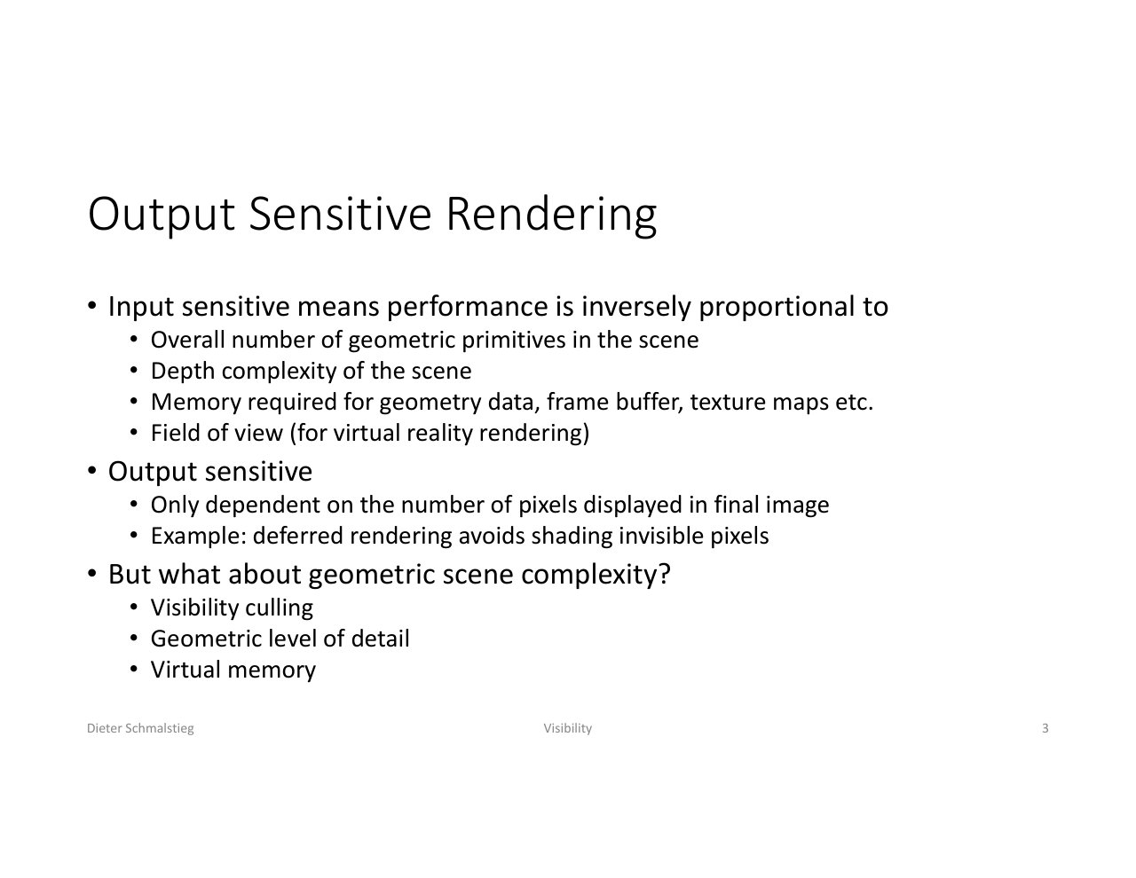
L14_Pg-03: Input-sensitive performance scales with scene primitives, depth complexity, memory, and field of view; output-sensitive performance depends only on the pixels displayed.

Input-sensitive rendering means performance degrades with properties of the input scene: overall number of geometric primitives, depth complexity, memory for geometry, frame buffer, and textures, and (for VR) field of view. Output-sensitive rendering depends only on the number of pixels displayed in the final image.

Deferred rendering is output-sensitive for shading: it avoids shading invisible pixels. But geometric scene complexity remains input-sensitive, and three technique families attack it: visibility culling (this lecture), geometric level of detail (previous lecture), and virtual memory (next lecture).

2. Why the Z-Buffer Is Not Enough

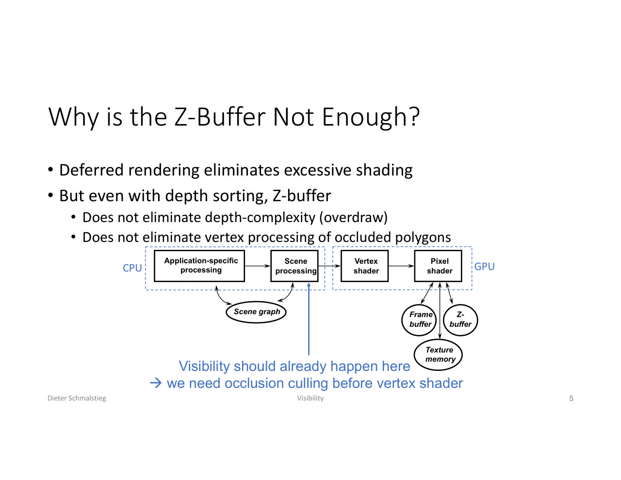
L14_Pg-05: The z-buffer sits at the end of the pipeline; occluded geometry has already gone through vertex processing and rasterization. Occlusion culling must happen before the vertex shader.

The depth buffer is hardware that determines per-pixel visibility: a 2D buffer of z-values per pixel, and a fragment result is stored only if the depth test passes. It allows drawing unsorted geometry, though sorting still helps: early-z testing runs the depth test before the pixel shader, so drawing near objects first increases the chance that later fragments are rejected before shading.

Even so, with deferred rendering eliminating excessive shading and with depth sorting, the z-buffer:

• does not eliminate depth complexity (overdraw: occluded fragments are still rasterized),
• does not eliminate vertex processing of occluded polygons.

Visibility should be resolved earlier: occlusion culling must happen before the vertex shader, on the CPU side or in a scene-processing pass.

3. The Three Culling Types

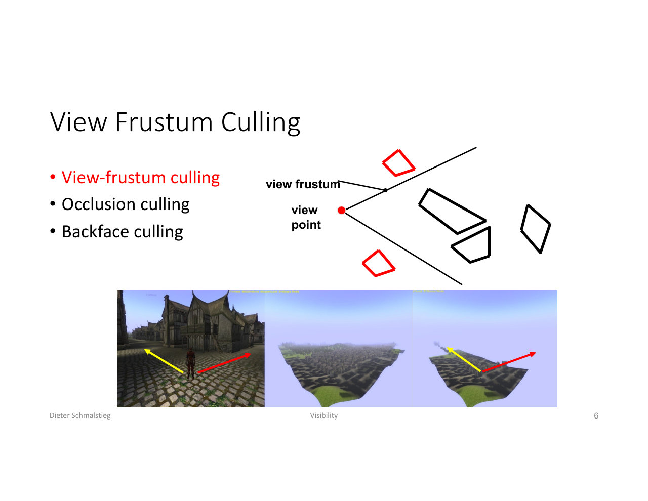
L14_Pg-06: View-frustum culling removes everything outside the camera's viewing volume.

Three cullers, in increasing order of difficulty:

1. View-frustum culling: discard objects outside the camera’s frustum.
2. Backface culling: discard primitives facing away from the camera.
3. Occlusion culling: discard objects hidden behind other objects.

View-Frustum Culling with a BVH

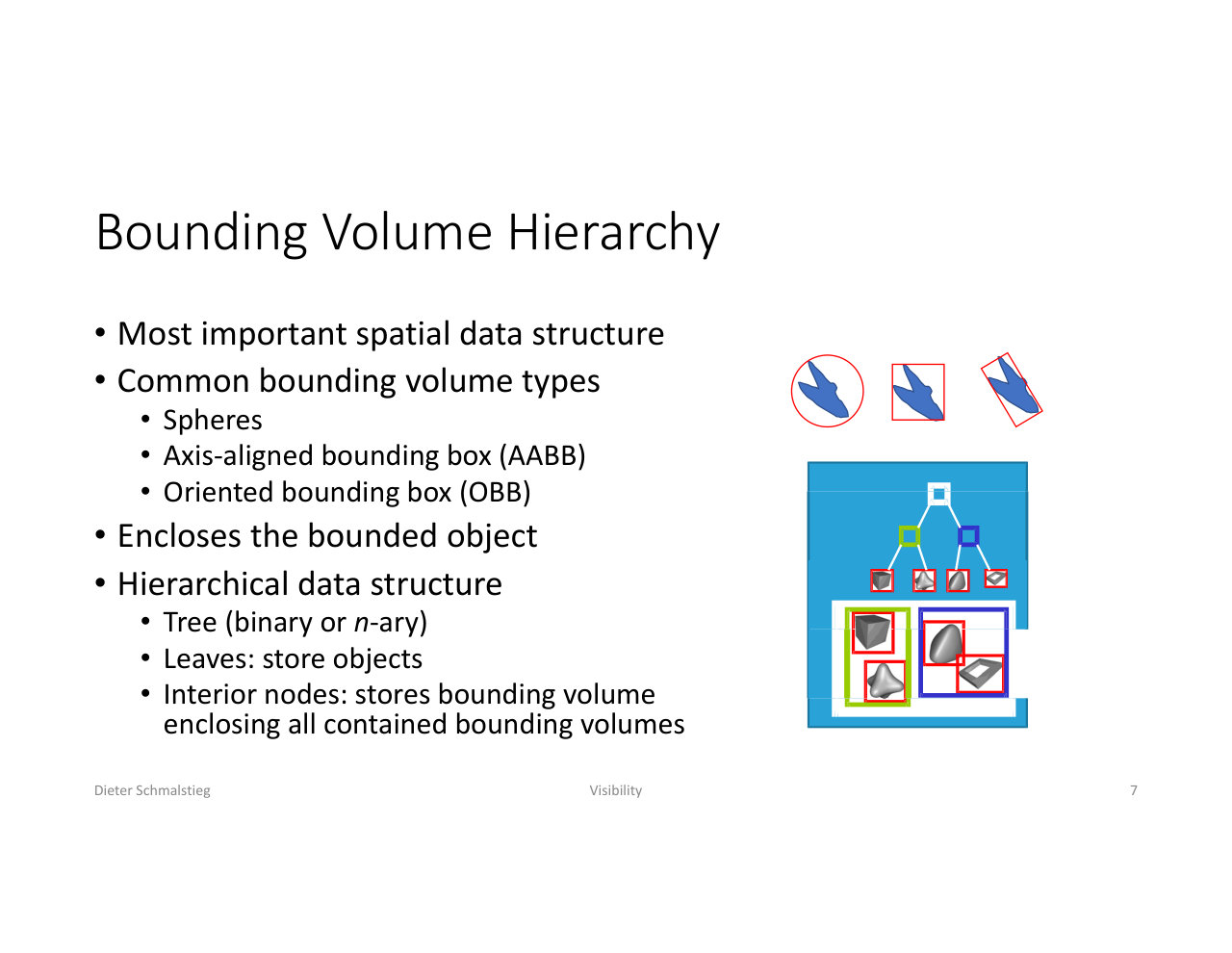
L14_Pg-07: The bounding volume hierarchy is the most important spatial data structure - spheres, AABBs, or OBBs in a tree whose interior nodes enclose all their children, leaves store the objects.

The bounding volume hierarchy (BVH) is the most important spatial data structure. Common bounding volumes: spheres, axis-aligned bounding boxes (AABB), oriented bounding boxes (OBB). The hierarchy is a binary or n-ary tree: leaves store objects, interior nodes store a bounding volume enclosing all contained volumes. Frustum culling then recurses only into intersected nodes:

Cull(node):
    if intersect(node, frustum) != EMPTY
        if node = LEAF then draw(node)
        else for all children C of node: Cull(C)

A single test against a high node can discard thousands of objects at once.

Backface Culling

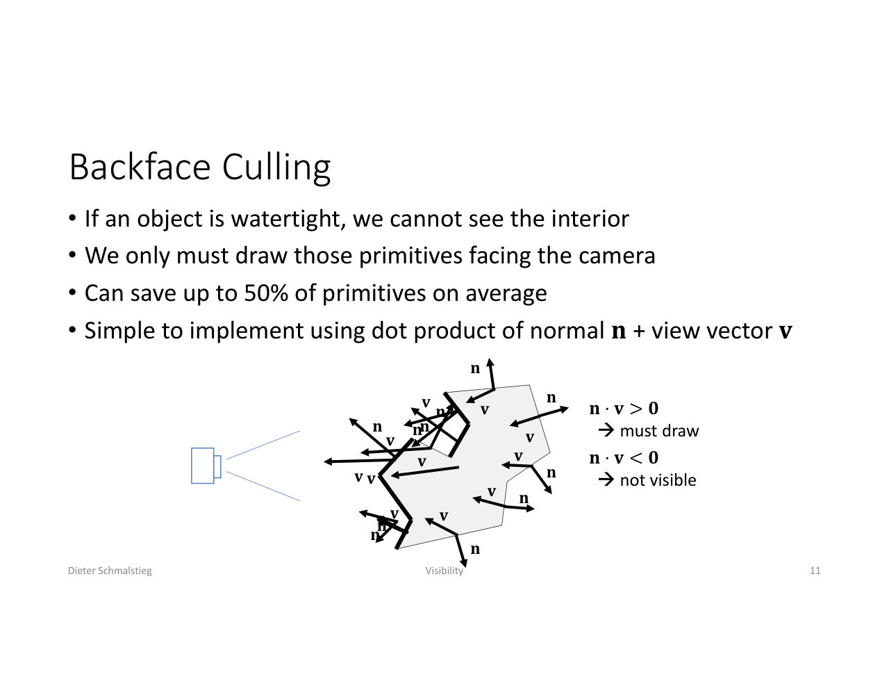
L14_Pg-11: For watertight objects only camera-facing primitives must be drawn; the sign of the dot product of normal and view vector decides, saving up to 50% of primitives on average.

If an object is watertight, its interior can never be seen, so only primitives facing the camera must be drawn. The test is the dot product of surface normal $\mathbf{n}$ and view vector $\mathbf{v}$: draw if $\mathbf{n}\cdot \mathbf{v}>0$, cull if $\mathbf{n}\cdot \mathbf{v}<0$ (with the lecture’s convention for the view vector). On average this saves up to 50% of primitives.

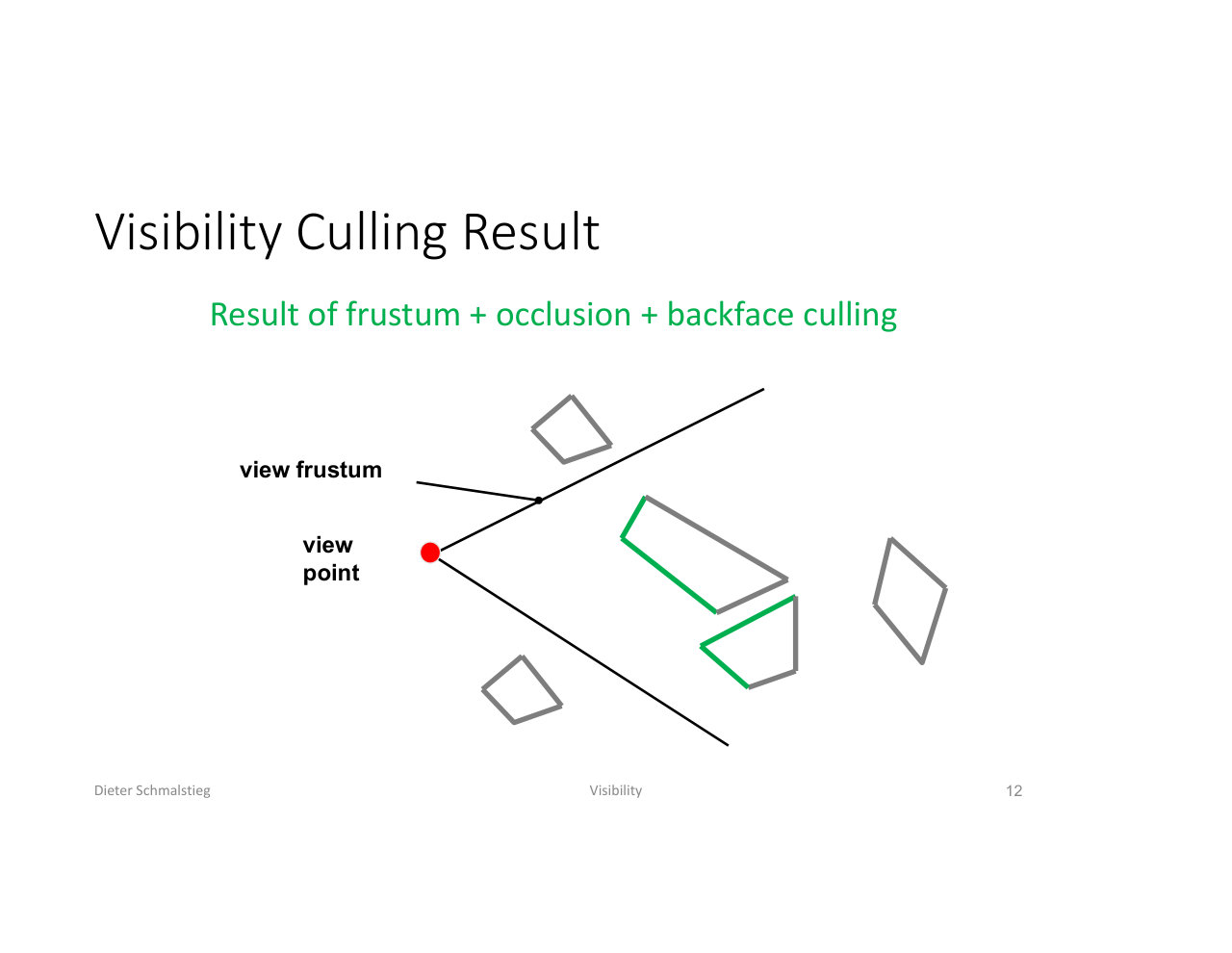
L14_Pg-12: The combined result of frustum, occlusion, and backface culling - only the primitives that can actually contribute to the image survive.

4. Exact vs. Potentially Visible Sets

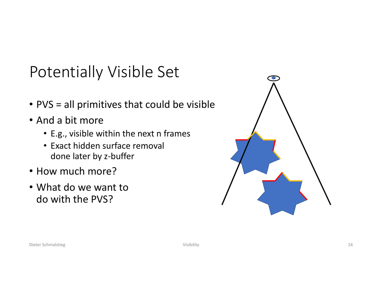
L14_Pg-14: The PVS contains everything that could be visible, and a bit more (for example, visible within the next n frames); exact hidden-surface removal is left to the z-buffer.

The Exactly Visible Set (EVS) contains all primitives that are visible, no more and no less. Computing it is impractical. Instead one computes a Potentially Visible Set (PVS): all primitives that could be visible, and a bit more, for example everything visible within the next $n$ frames. The z-buffer performs exact hidden-surface removal on whatever the PVS lets through.

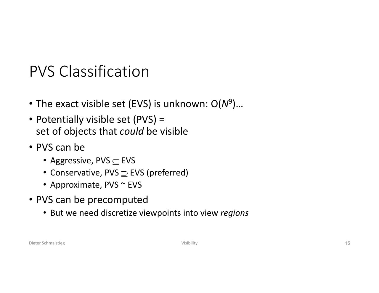
L14_Pg-15: PVS classification - aggressive (subset of EVS), conservative (superset, preferred), approximate (roughly equal). Precomputing a PVS requires discretizing viewpoints into view regions.

A PVS relative to the EVS can be:

• Aggressive: PVS ⊆ EVS. Fast, but can wrongly cull visible geometry (visible errors).
• Conservative: PVS ⊇ EVS. Preferred: never wrong, just some wasted work.
• Approximate: PVS ≈ EVS. Errors in both directions.

A PVS can be precomputed, but then viewpoints must be discretized into view regions (section 8).

5. Occlusion Culling from a Point

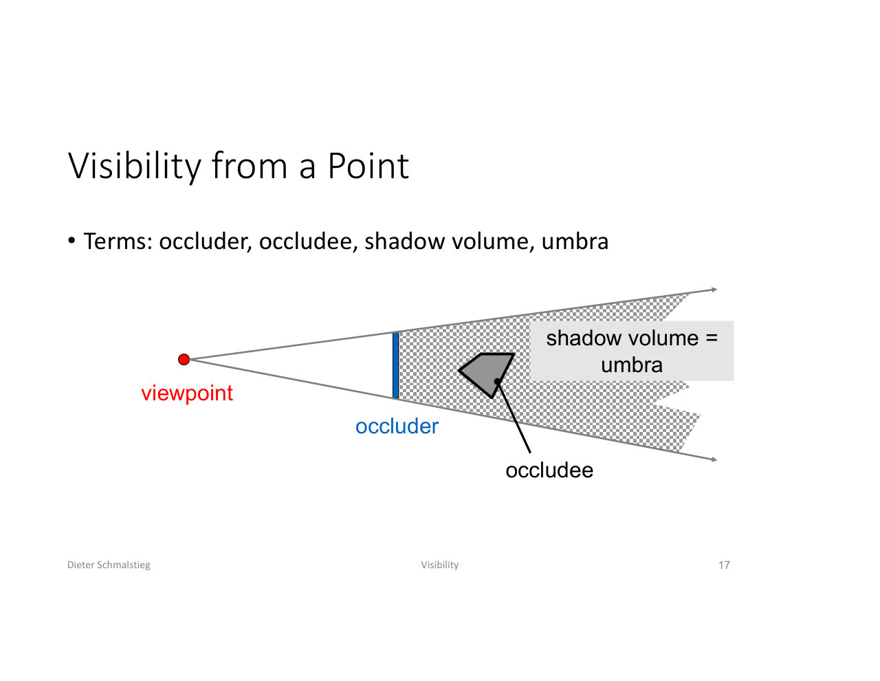
L14_Pg-17: Vocabulary of point visibility - the occluder casts a shadow volume (umbra) from the viewpoint; any occludee fully inside the umbra is invisible.

A naive occlusion culler selects a few promising occluders (large objects, close to the camera so they are large in screen space), tests all other objects against them, and removes the occluded ones, perhaps testing bounding boxes instead of the objects. This does not work well for real-life scenes, because single objects rarely occlude much on their own; occlusion in realistic scenes comes from the combined effect of many occluders.

The vocabulary: an occluder casts a shadow volume (its umbra) from the viewpoint; an occludee inside that volume is hidden. For multiple occluders $oc{c}_1,\dots ,oc{c}_n$ the complete shadow volume is the union of the individual shadow volumes.

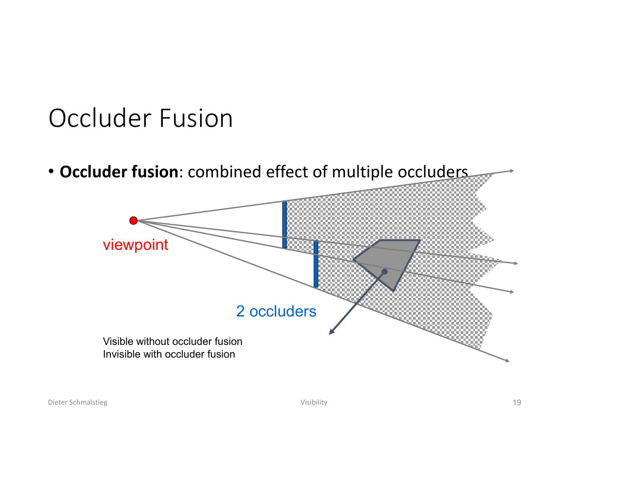
L14_Pg-19: Occluder fusion - an object invisible only through the combined effect of two occluders is missed when occluders are tested individually.

Occluder fusion is the crucial idea: capturing the combined effect of multiple occluders. An occludee may be visible with respect to every single occluder yet invisible behind their union.

The Practical Structure

In practice occlusion culling uses two spatial data structures:

1. the scene data structure (SDS) storing the objects of the scene,
2. the shadow volume data structure (SVDS), generated from selected occluders or from synthesized virtual occluders.

The SDS is culled against the SVDS. The basic point-visibility algorithm:

SVDS = empty
for each occluder occ_i:
    calculate shadow volume SV_i
    add SV_i to SVDS
for every object o_j:
    test o_j against the SVDS
    cull o_j if occluded

Spatial Data Structures

For quickly culling large portions of the scene with a single test, all kinds of hierarchical structures are used: bounding boxes, BVHs, grids, quadtrees, octrees (the 3D equivalent of a quadtree, hierarchically subdividing a cube into 8 octants), k-d trees, BSP trees.

6. Cells and Portals

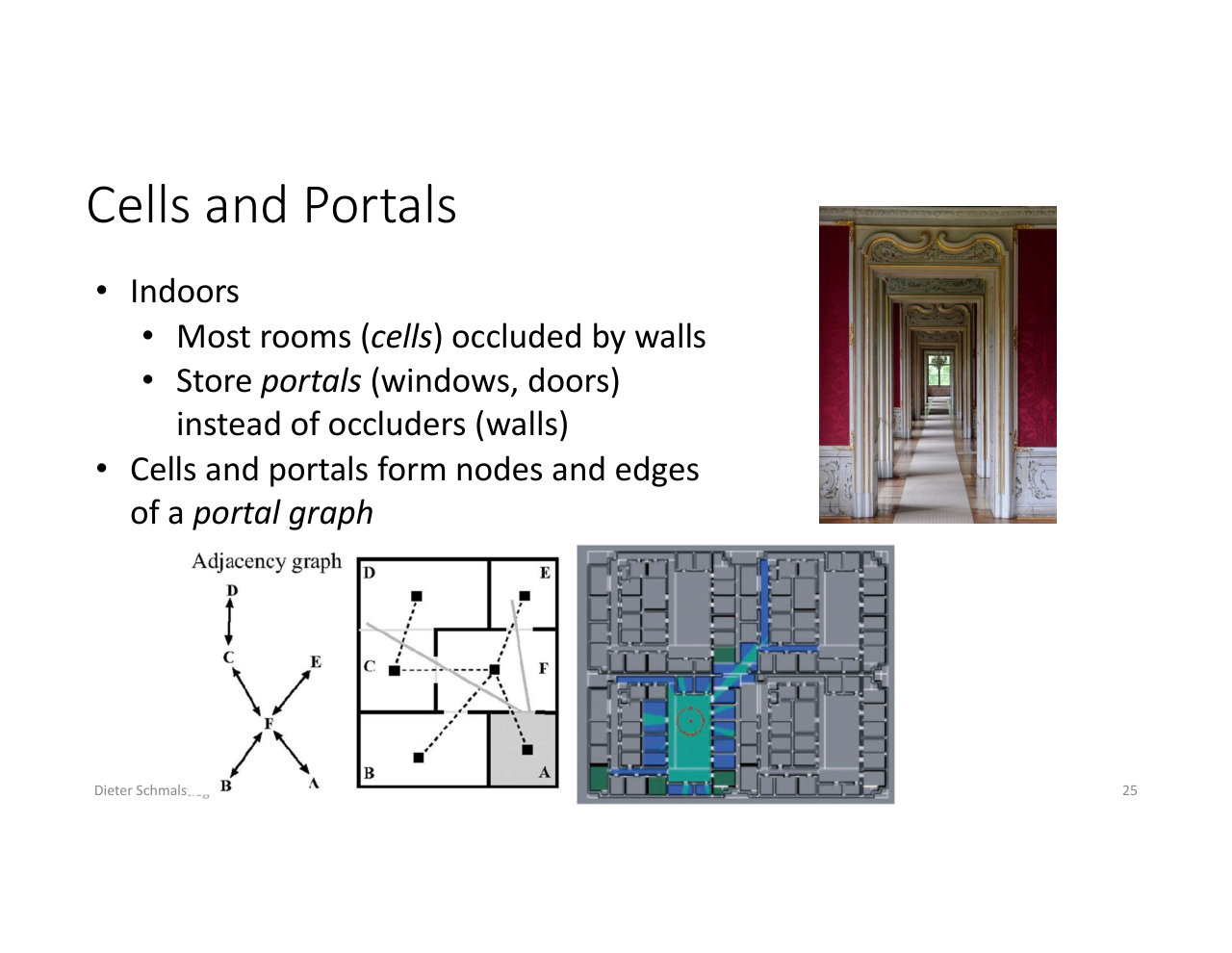
L14_Pg-25: Indoors, rooms are cells occluded by walls; storing the portals (doors, windows) instead of the occluders turns the scene into a portal graph of cells and openings.

Indoors the occlusion structure is special: most rooms (cells) are occluded by walls. Instead of storing the walls as occluders, store the portals (windows, doors) through which anything can be seen. Cells and portals form the nodes and edges of a portal graph.

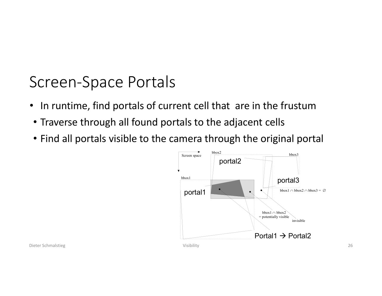
L14_Pg-26: Screen-space portal traversal - starting from the current cell, portals in the frustum are traversed into adjacent cells, intersecting portal bounding rectangles in screen space until nothing remains visible.

At runtime: find the portals of the current cell that are inside the frustum, traverse through each found portal to the adjacent cell, and find the portals visible through the original portal, intersecting their screen-space bounding rectangles. Where the intersection becomes empty, traversal stops; everything beyond is invisible.

7. Depth-Buffer-Based Occlusion Culling

Modern engines derive occlusion directly from depth information:

• Regular depth buffer / depth prepass: in deferred rendering, pass 1 rasterizes the geometry writing only depth and object id to the G-buffer; pass 2 reads and collects all visible ids. Exact, but can be expensive for large scenes with many primitives and high framebuffer resolutions.
• Virtual occluders: objects with many primitives are expensive occluders, and bounding volumes cannot be used because they are not conservative (they occlude more than the object). Instead use bounded volumes completely contained inside the object; these virtual occluders can be simple boxes.

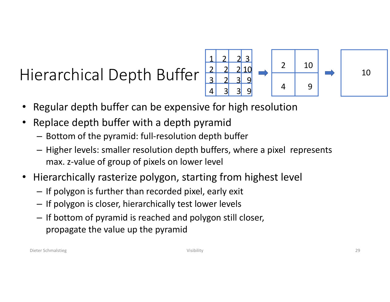
L14_Pg-29: The hierarchical depth buffer replaces the depth buffer with a max-z pyramid; polygons are tested top-down and rejected early if they are farther than the recorded pixel.

• Hierarchical depth buffer (Hi-Z): a full-resolution depth buffer is expensive to test against, so replace it with a depth pyramid. The bottom level is the full-resolution depth buffer; each higher level stores, per pixel, the maximum z-value of the corresponding group of pixels below. A polygon is rasterized hierarchically from the top: if it is farther than the recorded value, early exit (occluded); if closer, descend and test the lower levels; if it reaches the bottom still closer, its depth is written and propagated up the pyramid. Whole polygons die after a handful of coarse tests.

💡 Intuition

Hi-Z is to the z-buffer what the BVH is to the object list: the same test, made logarithmic by a hierarchy of conservative summaries. The pyramid stores max-z because that is the conservative direction, being behind the farthest recorded depth in a whole region proves occlusion for every pixel of that region at once.

8. Visibility from a Region

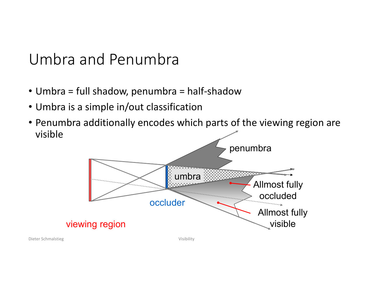
L14_Pg-31: From a viewing region, an occluder casts an umbra (fully hidden from every viewpoint) and a penumbra (hidden from some viewpoints); only the umbra proves invisibility.

Precomputing visibility requires discretizing viewpoints into view regions, and it only works for static scenes. From a region, an occluder casts:

• an umbra (full shadow): invisible from every viewpoint of the region, a simple in/out classification,
• a penumbra (half shadow): additionally encodes which parts of the viewing region see it.

Only the umbra can be used for conservative culling.

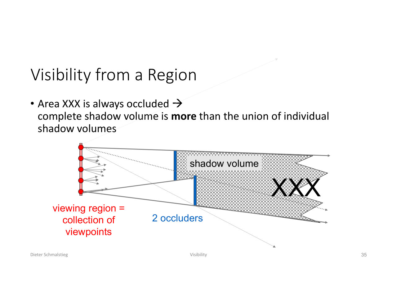
L14_Pg-35: The region XXX is always occluded by the two occluders together, even though it lies in neither individual umbra - the complete shadow volume of a region is more than the union of the individual volumes.

The subtlety of region visibility: an area can be occluded from every single viewpoint of the region without lying in the umbra of any single occluder. The complete shadow volume is more than the union of individual shadow volumes, so occluder fusion is even more important than in the point case.

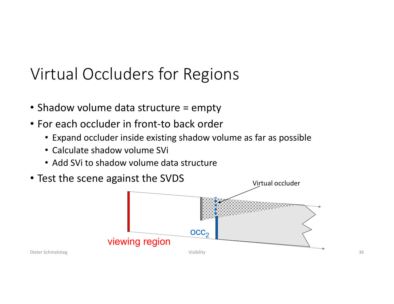
L14_Pg-36: Virtual occluders for regions - processing occluders front to back and expanding each occluder as far as possible inside the existing shadow volume captures fused occlusion conservatively.

Virtual occluders for regions capture this fusion:

SVDS = empty
for each occluder in front-to-back order:
    expand occluder inside existing shadow volume as far as possible
    calculate shadow volume SV_i
    add SV_i to SVDS
test the scene against the SVDS

Because an occluder may be expanded through space that is already inside the accumulated shadow volume, the umbrae of separate occluders merge. Koltun, Chrysanthou, and Cohen-Or (2000) build such virtual occluders from fusion via an intermediate data structure: search inside the umbra for adjunct occluders and add them, growing a virtual occluder that is guaranteed occluded from the cell and can become very large. The virtual occluders are an efficient intermediate PVS representation.

🧠 Deep Dive: Where Nanite Fits

Unreal Engine 5’s Nanite uses the simplest possible occlusion strategy from this toolbox, applied aggressively: render first what was visible in the last frame (an excellent conservative guess under temporal coherence), build a hierarchical depth buffer from it, then test everything else against that Hi-Z pyramid. Combined with the view-dependent cluster LOD from the previous lecture and the virtualized textures and geometry of the next one, this is what makes “the end of polycounts” marketable.

---

Applied Exam Focus

• Input vs output sensitive: input-sensitive cost grows with primitives, depth complexity, memory, field of view; output-sensitive cost depends only on displayed pixels. Deferred shading fixed shading; culling, LOD, and virtual memory attack geometry.
• Z-buffer limits: exact per-pixel visibility, early-z helps, but overdraw and vertex processing of occluded polygons remain; occlusion culling must happen before the vertex shader.
• Three cullers: view frustum (BVH recursion), backface ($\mathbf{n}\cdot \mathbf{v}$ sign test, watertight objects, up to 50% savings), occlusion (the hard one).
• EVS vs PVS: EVS impractical; PVS aggressive (⊆), conservative (⊇, preferred), approximate (≈). Precomputed PVS needs view regions and static scenes.
• Point visibility: occluder, occludee, shadow volume, umbra; union of volumes; occluder fusion for combined effects; SDS culled against SVDS.
• Cells and portals: indoor scenes, store openings instead of walls, portal graph, screen-space portal traversal.
• Depth-based: depth prepass with object ids; virtual occluders as boxes inside objects (bounding volumes are not conservative); hierarchical depth buffer with max-z pyramid and top-down early rejection.
• Region visibility: umbra vs penumbra; the complete shadow volume exceeds the union of individual umbrae; virtual occluders expanded front-to-back inside the accumulated volume capture fusion (Koltun et al. 2000).

Self-Check

1. Define input-sensitive and output-sensitive rendering, and name the three technique families that make geometry handling output-sensitive.

Answer

Input-sensitive means performance is proportional to input scene properties: total number of primitives, depth complexity, memory for geometry/framebuffer/textures, and field of view in VR. Output-sensitive means performance depends only on the number of pixels displayed in the final image. Deferred rendering already avoids shading invisible pixels; for geometric complexity the three families are visibility culling, geometric level of detail, and virtual memory.

2. The z-buffer already computes exact visibility. Why is occlusion culling still needed, and where must it happen?

Answer

The z-buffer resolves visibility per pixel only at the end of the pipeline. Even with depth sorting and early-z, it does not eliminate overdraw (occluded fragments are still rasterized) and does not eliminate vertex processing of occluded polygons: all that work is already spent by the time the depth test runs. Occlusion culling therefore has to happen before the vertex shader, during scene processing.

3. How does frustum culling with a BVH work, and why is it fast?

Answer

The BVH is a tree whose leaves store objects and whose interior nodes store a bounding volume (sphere, AABB, or OBB) enclosing all contained volumes. Culling recursively tests nodes against the frustum: if a node does not intersect the frustum, its entire subtree is discarded with that single test; if it intersects, recurse into the children, drawing intersected leaves. One test near the root can eliminate thousands of objects.

4. Classify PVS variants relative to the EVS. Which is preferred and why?

Answer

The exactly visible set (EVS) contains precisely the visible primitives but is impractical to compute. A PVS can be aggressive (PVS ⊆ EVS, may wrongly cull visible geometry, causing visible errors), conservative (PVS ⊇ EVS, never misses visible geometry, only wastes some work on invisible geometry), or approximate (PVS ≈ EVS, errors in both directions). Conservative is preferred: correctness is guaranteed and the z-buffer cleans up the extra, invisible primitives that slipped through.

5. What is occluder fusion and why does naive occlusion culling fail without it?

Answer

Occluder fusion is capturing the combined occlusion effect of multiple occluders. Naive culling selects a few large, close occluders and tests objects against each individually; it fails on real scenes because single objects rarely hide much on their own. An occludee can be visible with respect to every individual occluder yet lie completely hidden behind their union. In the region-visibility case fusion matters even more, because the complete shadow volume of several occluders is more than the union of their individual shadow volumes.

6. Describe the hierarchical depth buffer and its culling test.

Answer

The depth buffer is replaced by a depth pyramid: the bottom level is the full-resolution depth buffer, and each higher level stores per pixel the maximum z-value of the corresponding group of pixels on the level below. A polygon is tested top-down: if it is farther than the recorded value at the current level, it is occluded and rejected early; if closer, the test descends hierarchically; if it reaches the bottom still closer, it is visible and its depth is written and propagated back up the pyramid. Occluded geometry dies after a few coarse tests instead of per-pixel comparisons.

7. Why can an object’s bounding volume not serve as an occluder, and what is used instead?

Answer

A bounding volume encloses the object, so it occludes more than the object actually does; using it as an occluder would cull objects that are really visible, which is not conservative. Instead one uses volumes completely contained inside the object (virtual occluders), which occlude at most what the real object occludes. They can be simple boxes, and detailed, primitive-heavy objects get cheap stand-in occluders this way.

8. How do cells and portals exploit indoor structure?

Answer

Indoors, most rooms (cells) are mutually occluded by walls. Rather than treating the many walls as occluders, the system stores the portals (doors, windows), the only openings through which other cells can be seen. Cells and portals form a portal graph. At runtime, the portals of the current cell inside the frustum are traversed into adjacent cells, and visibility continues only through the screen-space intersection of the portal rectangles along the path; when the intersection is empty, everything beyond is culled.

9. Distinguish umbra and penumbra for region visibility, and explain why precomputed region PVS requires static scenes.

Answer

From a viewing region, the umbra of an occluder is the space invisible from every viewpoint in the region (a simple in/out classification usable for conservative culling), while the penumbra is visible from some viewpoints and additionally encodes which parts of the region see it. Precomputing visibility requires discretizing all possible viewpoints into regions and computing shadow volumes offline; if occluders move, the precomputed umbrae become invalid, so the approach only works for static scenes.

---

Back: (y-13) Levels of Detail | RTG Index | Next: (y-15) Virtual Textures