13_lod - Levels of Detail

Back: (y-12) High Dynamic Range | RTG Index | Next: (y-14) Visibility

Mental Model First: Spend Polygons Where the Eye Can See Them

• Even after visibility culling, a scene can contain far more polygons than the frame budget allows. Level of detail (LOD) attacks this by rendering small or distant objects with simplified versions of their geometry.
• LOD has two independent halves: selection and generation. Selection decides at runtime which detail level each object gets (static, reactive, or predictive). Generation builds the simplified versions in the first place (subdivision, simplification operators, quadric error metrics).
• Switching between levels is its own problem. Hard switches pop, blending costs extra fill, and geomorphing interpolates geometry smoothly but needs correspondence between the levels.
• The end state of this line of thinking is continuous and view-dependent LOD, where the resolution varies inside a single object and the renderer always extracts exactly the polygon count it can afford. Unreal Engine 5’s Nanite is the industrial-strength version of this idea, combined with the visibility and virtual texture techniques of the next two lectures.

---

1. The Basic Idea

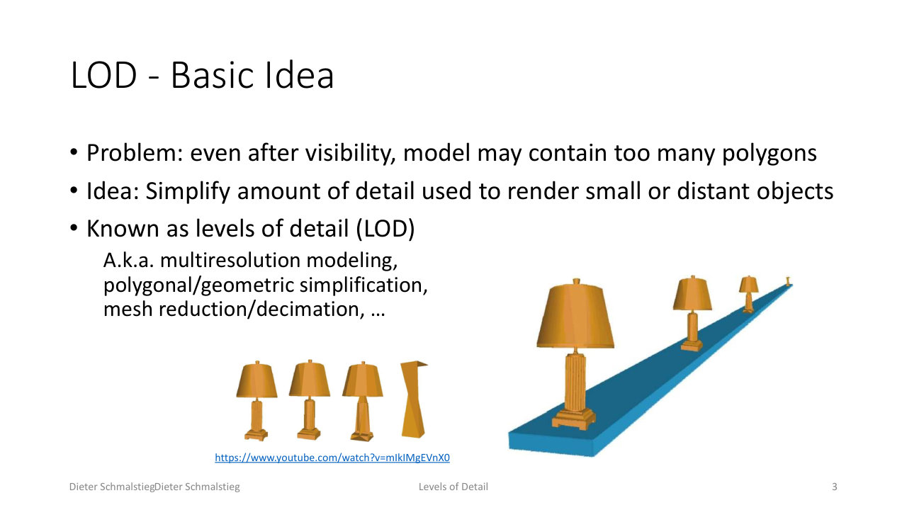
L13_Pg-03: Even after visibility culling the model may contain too many polygons, so small or distant objects are rendered with simplified detail.

The problem: even after visibility culling, the model may contain too many polygons for the frame budget. The idea: simplify the amount of detail used to render small or distant objects, since the screen cannot resolve that detail anyway. The technique goes under many names: levels of detail (LOD), multiresolution modeling, polygonal or geometric simplification, mesh reduction, mesh decimation.

2. Static LOD Selection

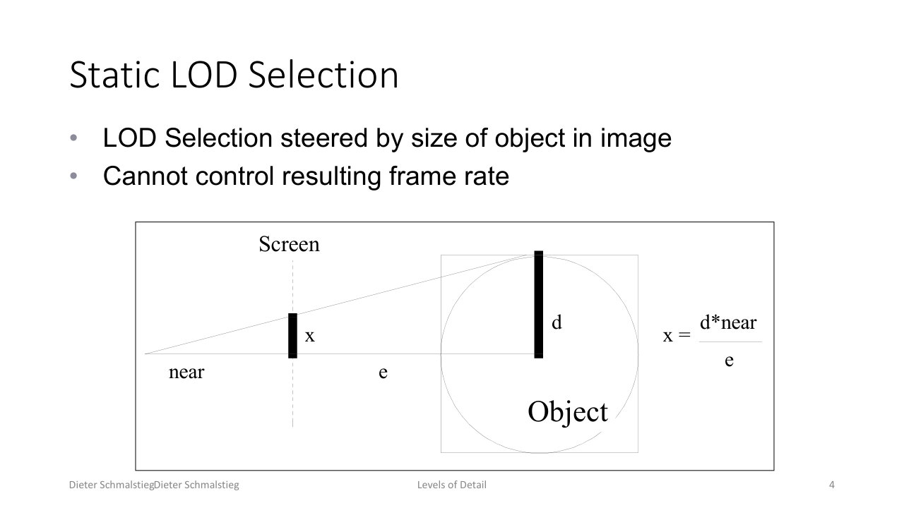
L13_Pg-04: Static selection picks the LOD from the projected size of the object on screen, x = e * near / d.

The simplest scheme selects the LOD based on the size of the object in the image. Projecting an object of extent $e$ at distance $d$ onto a screen at the near plane gives the projected size

$x=\frac{e\cdot near}{d}$

and thresholds on $x$ pick the level. The weakness: selection depends only on geometry, so it cannot control the resulting frame rate. A view full of large objects still overloads the GPU.

3. Reactive LOD Selection

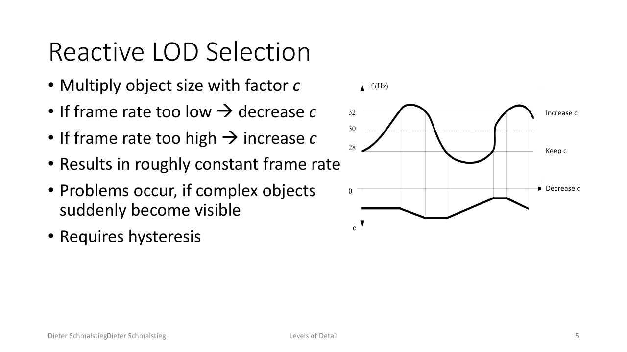
L13_Pg-05: Reactive selection scales object size by a factor c driven by the measured frame rate, with a hysteresis band between the overloaded and underloaded regimes.

Reactive selection closes a feedback loop over the frame rate. The projected object size is multiplied by a factor $c$:

• frame rate too low: decrease $c$ (coarser LODs everywhere),
• frame rate too high: increase $c$ (finer LODs).

This yields a roughly constant frame rate. Problems occur when complex objects suddenly become visible, because the controller only reacts after the slow frame has already happened. The controller also needs hysteresis (a dead band where $c$ stays unchanged) so it does not oscillate between levels.

4. Predictive LOD Selection

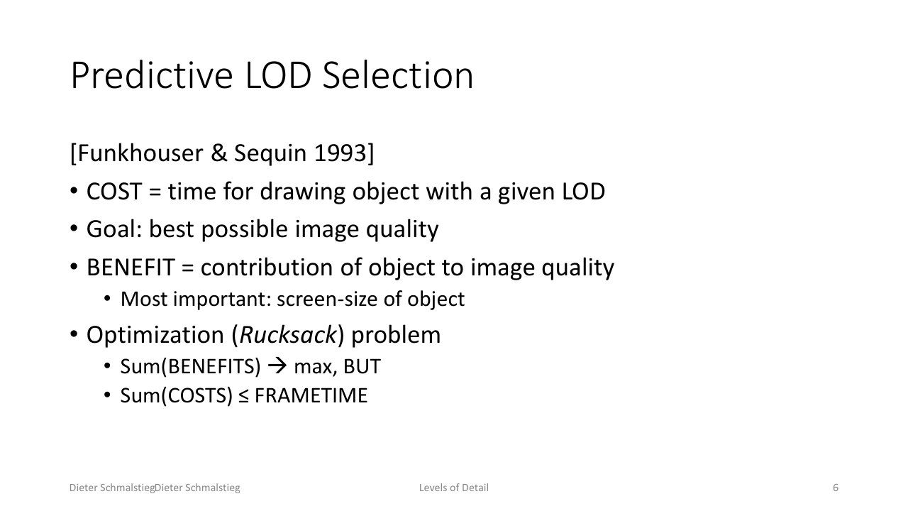
L13_Pg-06: Predictive selection (Funkhouser and Sequin 1993) treats LOD assignment as a knapsack problem: maximize summed benefit subject to summed cost staying within the frame time.

Predictive selection [Funkhouser & Sequin 1993] avoids reacting after the fact by modeling cost and benefit up front:

• COST = time to draw an object at a given LOD.
• BENEFIT = the object’s contribution to image quality, dominated by its screen size.

Selection becomes a knapsack (Rucksack) optimization problem: choose LODs so that $\sum \text{BENEFIT}\to \max$ subject to $\sum \text{COST}\le \text{FRAMETIME}$. This gives the best possible image quality for a guaranteed frame time, at the price of solving (approximately) an optimization problem per frame.

💡 Intuition

The three selection schemes form a ladder of control theory: static is open-loop (no feedback at all), reactive is closed-loop feedback (correct after the error), predictive is feed-forward (model the cost before the error happens). Each rung buys frame-rate stability at more computational and implementation cost.

5. LOD Switching

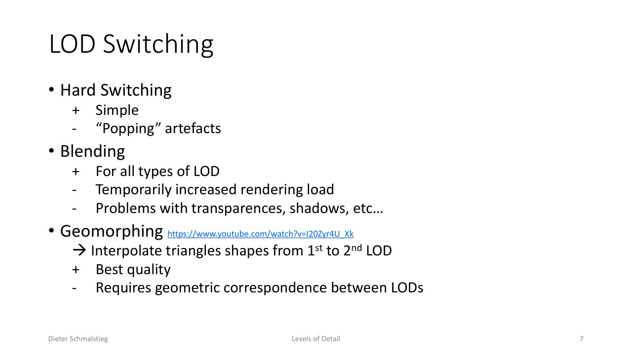
L13_Pg-07: Three switching strategies - hard switching pops, blending doubles the load during the transition, geomorphing interpolates vertices between the two levels.

Once the level changes, the transition must be hidden:

• Hard switching: simply swap models. Simple, but produces visible “popping” artifacts.
• Blending: cross-fade the two levels. Works for all types of LOD, but temporarily increases rendering load (both levels drawn) and causes problems with transparency, shadows, and similar effects.
• Geomorphing: interpolate the triangle shapes from the first LOD to the second. Best quality, but requires a geometric correspondence between the levels, which constrains how the LODs are generated.

6. Where LODs Come From

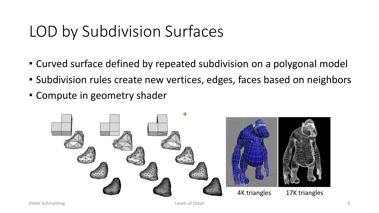
L13_Pg-08: Subdivision surfaces generate detail upward - repeated subdivision rules turn a 4K-triangle control mesh into a smooth 17K-triangle surface, computable in the geometry shader.

There are several ways to obtain the different detail levels:

• Subdivision surfaces work upward from a coarse mesh: a curved surface is defined by repeated subdivision of a polygonal model, with rules that create new vertices, edges, and faces from their neighbors. This can be computed in the geometry shader, so the coarse mesh is the asset and the detail is synthesized on the GPU.
• Shading and rendering LOD: detail reduction does not have to be geometric. Illumination can degrade from complex global to simple local models with distance, and geometry can be replaced by images (textures, impostors).
• Geometric simplification works downward from a detailed mesh, which is the classical path and the subject of the next sections.

7. Geometric Simplification

L13_Pg-10: Geometric simplification iteratively removes primitives; note that it does not change rasterization, so fragment shader load stays roughly identical.

Geometric simplification iteratively reduces the number of primitives (vertices, edges, triangles). A separate concern is topology simplification, which reduces the number of holes, tunnels, and cavities.

An important caveat: simplification reduces vertex processing, but it does not change rasterization. The object still covers the same pixels, so the fragment shader load remains roughly identical. LOD attacks the geometry side of the pipeline, not the fill side.

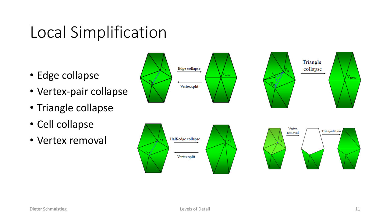
L13_Pg-11: The local simplification operators - edge collapse, vertex-pair collapse, triangle collapse, cell collapse, and vertex removal.

The atomic operations are local simplification operators:

• Edge collapse: merge the two endpoints of an edge into one vertex.
• Vertex-pair collapse: like edge collapse but for two vertices not connected by an edge (can merge separate components).
• Triangle collapse: collapse a whole triangle to a point.
• Cell collapse: merge all vertices in a spatial cell.
• Vertex removal: delete a vertex and retriangulate the hole.

Greedy Simplification

The standard driver is a greedy algorithm over a priority queue of operations ordered by error cost:

compute costs (error) for each possible operation
insert them into queue
while the queue is not empty
    extract head of queue (has smallest error)
    perform simplification operation

Each operation changes the costs of its neighbors, so a naive implementation constantly recomputes costs. The lazy greedy variant defers this with dirty flags:

compute costs for each possible operation
insert them into queue, set "dirty" flags to false
while the queue is not empty
    extract head of queue
    if head is dirty
        re-compute cost, clear dirty flag, re-insert into queue
    else
        perform simplification operation
        for each neighbor: set "dirty" flag to true

Costs are only recomputed when a stale entry actually reaches the head of the queue, giving far fewer cost evaluations.

8. The Quadric Error Metric

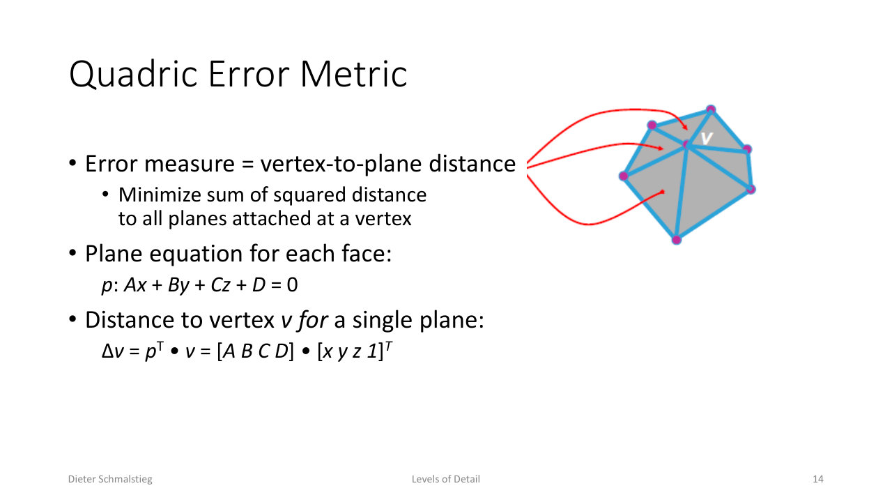
L13_Pg-14: The error measure is vertex-to-plane distance - each face contributes a plane p, and the distance of vertex v to that plane is the dot product pT v.

Which collapse is cheapest? The classic answer is the quadric error metric (QEM): the error of a vertex is the sum of squared distances to all planes attached at that vertex.

Each face defines a plane $p:Ax+By+Cz+D=0$. The signed distance of vertex $v$ to that single plane is

$\Delta v=p^T\cdot v=[ABCD]\cdot [xyz1{]}^T$

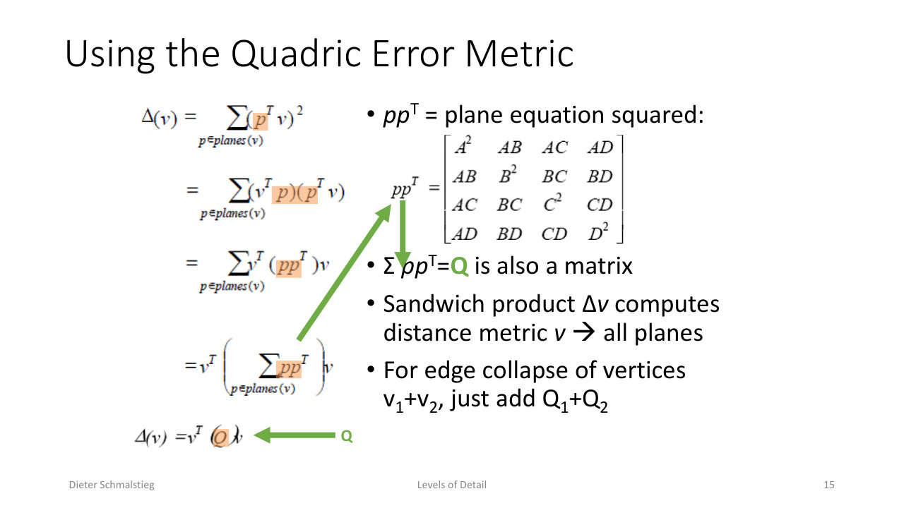
L13_Pg-15: Summing the outer products p pT over all planes gives a single 4x4 matrix Q; the sandwich product vT Q v evaluates the summed squared distance, and collapsing v1 and v2 just adds Q1 + Q2.

The squared distance to one plane is expressed with the outer product $p{p}^T$, a symmetric $4\times 4$ matrix. Summing over all planes at the vertex gives one matrix $Q=\sum p{p}^T$, and the sandwich product $v^{T}Qv$ evaluates the total squared distance of $v$ to all its planes at once. The killer feature: for an edge collapse of $v_1$ and $v_2$, the quadric of the merged vertex is just $Q_1+Q_2$. No plane lists have to be maintained, only $4\times 4$ matrices added.

Optimal Vertex Placement

Each vertex carries its quadric $Q$. Original vertices have zero error; vertices created by merges have nonzero error. Instead of placing the merged vertex at an endpoint or midpoint, one can minimize $Q$ to compute the optimal position for the new vertex. Empirically this gives 40 to 50 percent less error.

Boundary Preservation

Important boundaries would otherwise erode away. The fix: label edges as normal or discontinuity. For each face at a discontinuity, form a plane that perpendicularly intersects the discontinuous edge, convert those planes into quadrics too, and weight them more heavily in the error value. The penalty keeps simplification from pulling vertices off the boundary.

🧠 Deep Dive: Why QEM Won

QEM (Garland and Heckbert 1997) hits a sweet spot: the error model is geometrically meaningful (distance to the original surface’s tangent planes), the representation is constant-size (one symmetric 4x4 matrix per vertex, ten floats), the update under collapse is a single matrix addition, and minimizing the quadratic form for optimal placement is a small linear solve. Nearly every production simplifier since, including the offline preprocessing behind Nanite’s cluster hierarchy, is a descendant of this greedy-QEM skeleton.

9. Continuous and View-Dependent LOD

Discrete LODs waste quality at the switch points. Continuous LOD stores a data structure containing all LODs and extracts any desired one at runtime, so the renderer always uses the optimal polygon count and optimally exploits the available rendering power. Geomorphing then gives smooth transitions between the extracted levels.

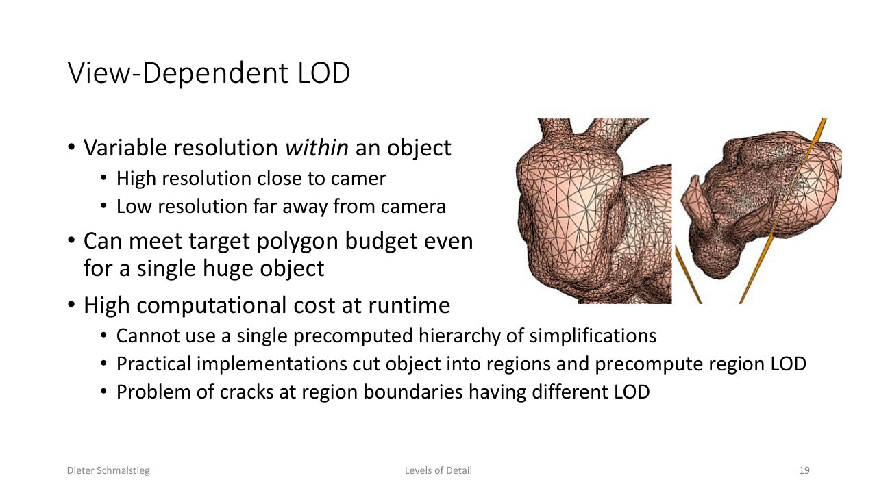
L13_Pg-19: View-dependent LOD varies resolution within one object - fine near the camera, coarse far away - which meets a polygon budget even for a single huge object, at high runtime cost.

View-dependent LOD goes further: the resolution varies within a single object, high close to the camera and low far away. This can meet a target polygon budget even for one huge object (a terrain, a massive statue). The costs:

• high computational cost at runtime,
• a single precomputed hierarchy of simplifications no longer suffices,
• practical implementations cut the object into regions and precompute per-region LODs,
• which creates the problem of cracks at region boundaries where adjacent regions use different LODs.

10. Terrain LOD

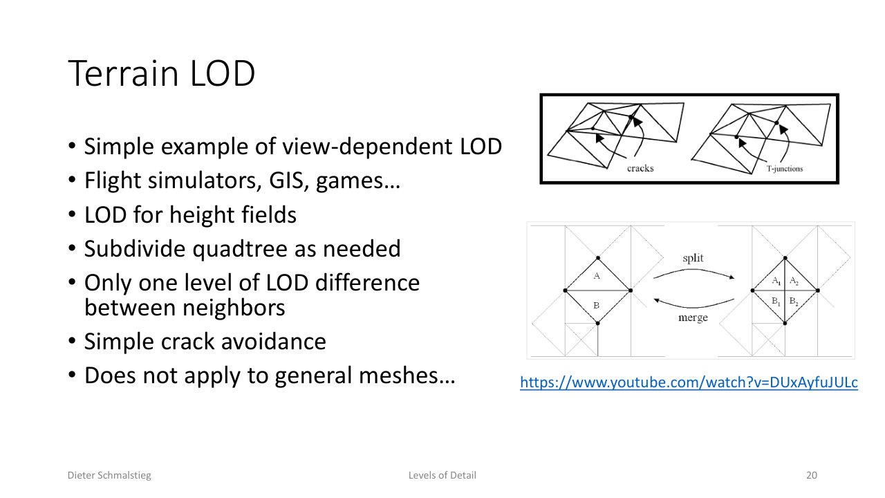
L13_Pg-20: Terrain LOD subdivides a quadtree over the height field as needed; allowing only one level of difference between neighbors gives simple crack avoidance.

Terrain is the classic, simple case of view-dependent LOD, used in flight simulators, GIS, and games. Because terrain is a height field, LOD reduces to subdividing a quadtree as needed near the viewer. Restricting neighbors to differ by at most one LOD level makes crack avoidance simple: the finer side can always be stitched to the coarser side. The catch is that this structure does not generalize to arbitrary meshes.

---

Applied Exam Focus

• Why LOD: after culling there can still be too many polygons; simplify small or distant objects. Also called multiresolution modeling, simplification, decimation.
• Selection: static (screen size $x=e\cdot near/d$, no frame-rate control), reactive (factor $c$ adjusted by frame-rate feedback, needs hysteresis, fails on suddenly visible objects), predictive (Funkhouser & Sequin: knapsack, maximize benefit subject to cost within frame time).
• Switching: hard (popping), blending (extra load, transparency/shadow problems), geomorphing (best quality, needs correspondence).
• Generation: subdivision surfaces (upward, geometry shader), shading/impostor LOD, geometric simplification (downward).
• Simplification does not reduce fragment load, only geometry load.
• Operators: edge collapse, vertex-pair collapse, triangle collapse, cell collapse, vertex removal; driven greedily by a cost queue, lazily with dirty flags.
• QEM: plane $p$, distance $\Delta v=p^{T}v$, quadric $Q=\sum p{p}^T$, error $v^{T}Qv$, collapse merges via $Q_1+Q_2$; optimal placement by minimizing $Q$ (40-50% less error); boundary preservation via weighted perpendicular planes on discontinuity edges.
• Continuous LOD: all levels in one structure, extract at runtime. View-dependent LOD: resolution varies inside one object, regions + precomputed LODs, crack problem.
• Terrain: quadtree over height field, max one level difference between neighbors for simple crack avoidance.

Self-Check

1. What problem does LOD solve that visibility culling does not, and what is the basic idea?

Answer

Visibility culling removes what is outside the frustum or occluded, but the remaining visible model may still contain too many polygons for the frame budget. LOD renders small or distant objects with simplified versions of their geometry, since the screen cannot resolve their full detail anyway. It is also known as multiresolution modeling, polygonal/geometric simplification, or mesh reduction/decimation.

2. Compare static, reactive, and predictive LOD selection.

Answer

Static selection picks the level from the projected screen size of the object, $x=e\cdot near/d$; it is simple but cannot control the resulting frame rate. Reactive selection multiplies object size by a factor $c$ and adjusts it by feedback: decrease $c$ when the frame rate is too low, increase it when too high. It holds a roughly constant frame rate but fails when complex objects suddenly appear and needs hysteresis to avoid oscillation. Predictive selection (Funkhouser & Sequin 1993) assigns each object-LOD pair a COST (draw time) and BENEFIT (contribution to image quality, mostly screen size) and solves a knapsack problem: maximize summed benefit subject to summed cost staying within the frame time.

3. What are the three LOD switching strategies and their trade-offs?

Answer

Hard switching swaps models instantly: simple, but produces popping artifacts. Blending cross-fades the levels: works for all LOD types, but temporarily increases rendering load and causes problems with transparency and shadows. Geomorphing interpolates the triangle shapes from one LOD to the next: best quality, but requires geometric correspondence between the levels.

4. Why does geometric simplification barely change fragment shader load?

Answer

Simplification reduces the number of primitives (vertices, edges, triangles), which cuts vertex processing. But the object still projects to the same pixels on screen, so rasterization is unchanged and the fragment shader runs roughly the same number of times. LOD is a geometry-side optimization, not a fill-rate optimization.

5. Explain the quadric error metric: what is measured, how is it represented, and why is it so cheap under edge collapse?

Answer

The error of a vertex is the sum of squared distances to all planes of the faces attached to it. Each face plane $p:Ax+By+Cz+D=0$ gives a distance $\Delta v=p^{T}v$ for homogeneous vertex $v$. Squaring is captured by the outer product $p{p}^T$, and summing these $4\times 4$ matrices over all attached planes gives one quadric matrix $Q$, so the total error is the sandwich product $v^{T}Qv$. Under an edge collapse of $v_1$ and $v_2$ the merged vertex’s quadric is simply $Q_1+Q_2$, a single matrix addition, with no plane lists to maintain.

6. How do optimal vertex placement and boundary preservation improve QEM simplification?

Answer

Optimal placement does not put the merged vertex at an endpoint or midpoint but at the position minimizing its quadric $Q$, which empirically reduces error by 40 to 50 percent. Boundary preservation labels edges as normal or discontinuity; for each face at a discontinuity a plane perpendicular to the discontinuous edge is formed, converted to a quadric, and weighted heavily, so collapses that would drag vertices off important boundaries become expensive and are avoided.

7. What is view-dependent LOD, why is it hard, and how does terrain get it cheaply?

Answer

View-dependent LOD varies the resolution within a single object: high near the camera, low far away, meeting a polygon budget even for one huge object. It is hard because it has high runtime cost and cannot use a single precomputed simplification hierarchy; practical systems cut the object into regions with precomputed region LODs, which creates cracks where neighboring regions differ in level. Terrain avoids most of this because a height field can be subdivided as a quadtree, and restricting neighbors to at most one level of difference makes crack avoidance simple. That trick does not apply to general meshes.

---

Back: (y-12) High Dynamic Range | RTG Index | Next: (y-14) Visibility